The Excel TRIM function is an amazing formula provided by Microsoft in its excel versions to remove extra spaces in a sentence in Excel. This function is very useful to clean the data by removing more than one space between two words in excel.
This function is very useful when you import some data from another application and the data is not in a proper format.
In this tutorial, we would unlock how to use the TRIM excel function along with examples.
Let us begin ! Here we go 😎
When To Use TRIM Function in Excel
As mentioned in the introduction, the TRIM formula in excel is used to remove all extra spaces between words in a cell in excel. It does, however, keep a single space between the words.
To put is simply, the TRIM function removes more than one space between text, and keep only single space. Additionally, it also removes spaces at the start and end of the text.
Also Read: How to Remove Leading Spaces in Excel
This function belong to the text function group, and therefore the it returns a text formatted value.
Syntax and Arguments
=TRIM(text)
The one and only argument of the TRIM function is text, explained below:
- text – In this argument, specify the text string (within double quotes) or a cell reference containing text in which you want to remove the extra spaces except one.
Examples of TRIM Excel Function Formula
In this section of the blog, let us look at some examples to understand how excel TRIM formula works.
Ex. 1 # Using TRIM Formula With Text
Below image contains some text with irregular spaces between the words.
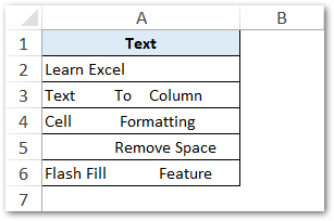
Let us now remove the all except one spaces from these texts using TRIM formula in excel.
In cell B2, simply type the following formula and copy it to other cells.
=TRIM(A2)
As a result, excel would remove more than one space characters as shown in the image below:
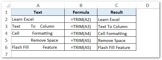
Ex. 2 # Using TRIM Formula With Numbers
In the above example, we learned how the TRIM formula works with texts. Let us now see how to TRIM numbers using the TRIM excel function.
Sample Data –
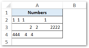
To trim the numbers in the above image, simply use the following formula in cell B2 and copy it to other cells in column B.
=TRIM(A2)
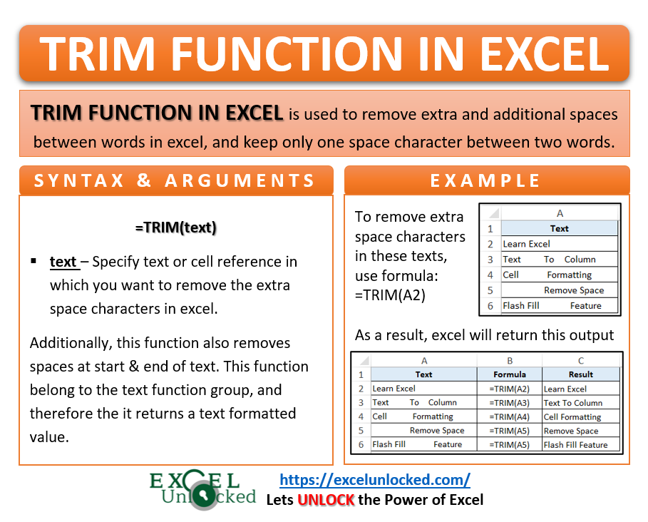
As a result, excel would return the following output.

In the above example, the excel keeps one space between numbers and removes all other space characters.
Remove All Spaces Between Words or Numbers in Excel
The TRIM function above removes all the additional spaces between words or numbers. However, this function keeps a single space.
Suppose now you want to remove all the spaces, such that all the words/number join each other, in the same data below:
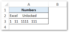
To achieve this, use the below formula in cell B2:
=SUBSTITUTE(TRIM(A2)," ","")
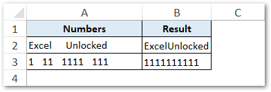
Explanation – In the above example, the TRIM function removes additional spaces and keep single space. The SUBSTITUTE function then replaces single space with blank.
You may also be interested to learn about –
With this, we have reached to the end of this blog. I hope this tutorial was useful for you !!
Thank You 🙂
