Many a time, you may have a dataset in excel wherein there is one additional character at the beginning of the dataset and you wish to remove this first character from those cells. Have you ever wondered how can we remove these unwanted first characters from these cells in Excel? There are multiple ways that you can use to achieve the same.
For Example, you have sample data wherein there is an exclamation mark ‘!’ followed by a number in Excel are numbers.
Now, you wish to remove the exclamation marks ‘!’ at one go from all the numbers.
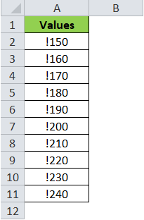
There are multiple ways which can be used to remove the first character from the cell or cells :
- Using “Find and Replace” functionality
- Formula based Approach : =REPLACE()
- Formula based Approach : =RIGHT()
- “Text to Column” functionality
Without wasting much time, let us discuss each of these methods one by one.
Remove First Character From Cell Using “Find and Replace”
By using this method, we are going to just replace the exclamation mark (!) with blank.
Follow the below steps to replace the exclamation mark with blank.
Select the dataset as shown in the screenshot below :
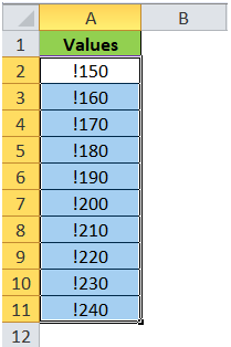
Open the “Find and Replace” dialog box by pressing Ctrl +H on your keyboard (Press Control key followed by H).
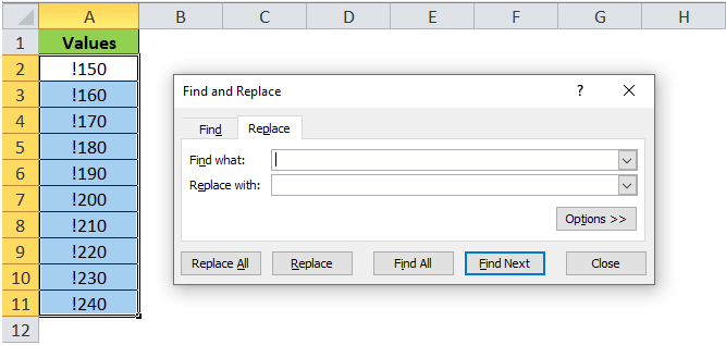
In the “Find What” section of this dialog box, enter the exclamation sign (i.e. !). And keep the “Replace With” section as it is. Do not enter anything over there.
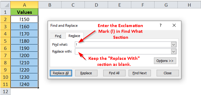
And click on the “Replace All” button.
Finally, you now have only the numbers in column A. The unwanted character (exclamation mark !) got removed.
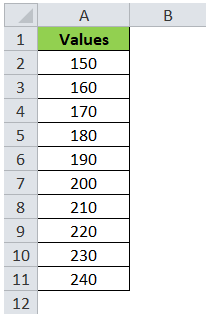
This method is useful only when the first character in all the cells is the same. In the present case, as the first character in all the cells is ! (i.e. same), hence we succeeded in removing it using the “Find and Replace” functionality of excel. This method would not work if there are homogeneous first characters in the range of cells.
Remove First Character From Cells Using Formulas
=REPLACE() formula
This is a formula based approach that would help to remove the first character from the string.
Unlike the first method, this method works even when the first character in the cell string is different.
Enter the below in cell B2 as shown in the screenshot:
=REPLACE(A2,1,1,””)
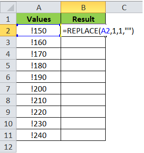
Press the “Enter” key on your keyboard.
As a result, you would notice that in cell A2 you have the string without first character.
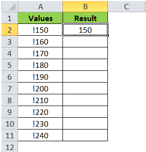
Copy the cell A2 and paste it to the other cells in column B to remove the first character (!) from all the values.
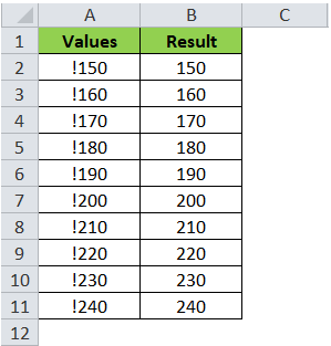
Explanation of the formula :
The first attribute of this formula is the text/string. In our case, it is A2.
The second and the third attribute of this formula is the start number and the number of characters to be replaced. In our case, the start number would be 1 and the number of characters will be 1 as we only want to remove the first character.
The fourth and the last attribute of this formula is the replacement text. In our case, it would be blank i.e. “” as we want to replace with nothing.
=RIGHT() formula
This is also a formula-based approach. Enter below in B2.
=RIGHT(A2,LEN(A2)-1)
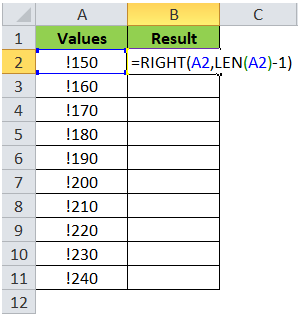
As soon as you press the “Enter” key on your keyboard, you would notice that the first character “!” got removed from the string.

Now copy the cell B2 and paste it to the other cells in column B.

Explanation of the Formula :
The =RIGHT() formula returns the specified number of characters from the right of the cell.
The first attribute of the formula is the text from which we want to return the characters from the right. In our case, it is cell A2.
The second attribute of this formula is the number of characters from the right of the text (the first character). We have used the formula LEN(A2)-1 as the second attribute of the =RIGHT() formula. LEN(A2)-1 depicts the numbers of characters in cell A2 reduced by 1. In our case, the LEN(A2)-1 would return the value as 3.
In a nutshell, the formula =RIGHT(A2,LEN(A2)-1) means that excel would return three characters from the right of the text specified in cell A2.
“Text to Column” functionality
The Text to Column functionality is the easiest method among all the above methods. The reason being, no formula is used in this method.
This method is also suitable in the case where the first character is different in each of the cells.
Excel has provided with a wizard to perform some steps.
Let us now, understand this method step by step :
Step 1: Select the range of cells as shown in the screenshot below :
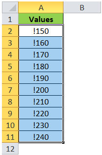
Step 2: Go to the “Data” tab. Under the “Data Tools” group select the option “Text to Column”.

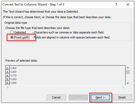
The Convert Text to Columns Wizard would appear on your screen.
Step 3: In the “Original Data Type” section, select the radio button “Fixed Width” and then click on the button ‘Next’.
Step 4: In the second step of this wizard, under the “Preview” section, rover your mouse to the ruler and click just between the first and the second character.
You would notice a vertical line after the first character as demonstrated in the screenshot below :
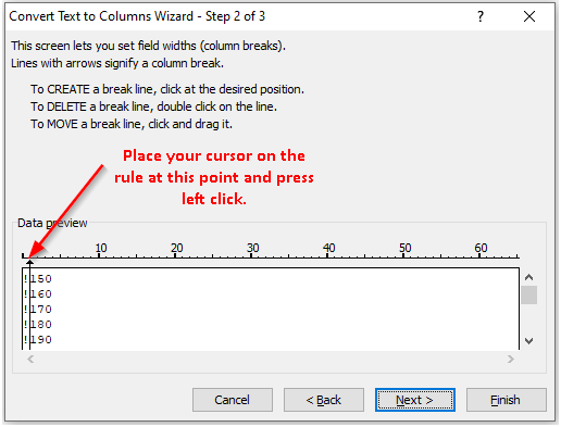
Now click on the “Next” button.
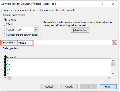
Step 5: Enter the destination location as cell B2 and finally click on the button – ‘Finish’
As a result, you would notice that the exclamation marks and the last three characters got separated in column B and column C respectively.
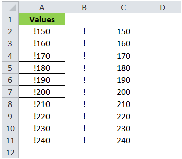
To get the values in column C in column A, simply copy the values in column C and paste it to column A. and then delete the values in columns B and C.
This brings us to the end of this blog.

