The Power Query Excel feature is a magical tool available inbuilt in newer excel versions. This tool assists excel users to import data and tables from internal and external sources, such as the same excel workbook, or other excel workbooks, JSON file, PDF, CSV or Text file, and many more. In addition to importing data, you can also do many transformations on this imported data using the power query tool. Splitting Cells is one of such transformation activity. In this blog, we would answer a very common question – ‘How to Split Cells or Columns in Excel Using Power Query‘ 🙂
The Excel power query feature has many more advantages. Check our overview blog to get insights about the basics and advantages of the power query feature in excel.
Sample Data for Splitting Columns in Excel
Have a look at the below sample data in the Excel Table.
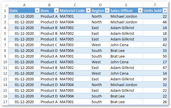
The above data is just an extract from 1000s of rows of excel table. Column E (Sales Officer) of this table contains the full name of the Sales Officers. Now, we want to split the first and last name from this full name into different columns in Excel.
One of the several ways is to create complex excel formulas using LEFT, FIND, LEN, and RIGHT excel function like shown in this blog.
But, why to use complex excel formulas when the power query split column feature can help you to achieve the desired result.
Split Cells or Columns in Excel [Step by Step Guide]
Before starting with the steps to split cells in excel, it is important to note that the Power Query feature only understands and imports the dataset which is in a proper excel table format. To convert a normal table into an excel table, simply select the dataset range, and use the keyboard shortcut ‘Ctrl + T’. In the dialog box that appears, click OK.
Once your dataset table is in a proper excel table format, you would see a new tab ‘Table Design’ on the excel ribbon. Change the name of the table as per your wish (for example – Split_Col).

Now, we are good to start with splitting the columns in this table.
- Click anywhere on the table and navigate to Data tab > Get & Transform Data group > Get Data > From Other Sources > From Table/Range as shown below:
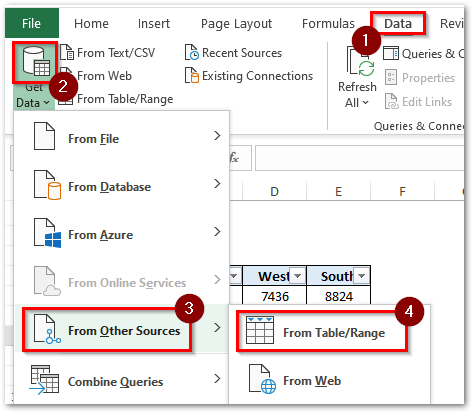
- As a result, excel would show the table data in the new window – ‘Power Query Editor’ window. Also, it would detect the data type for column header based on the first 200 rows of the data in the table. If not correctly detected, then you can change the data types and correct them.
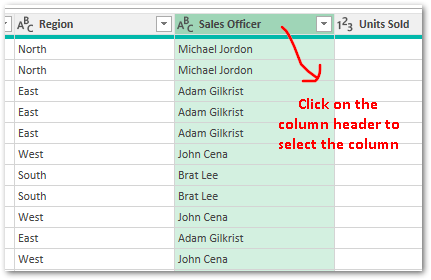
- Now, let us split the full names column ‘Sales Officer’ into first name and last name. Firstly, left-mouse click on the header ‘Sales Officer’ to select it.
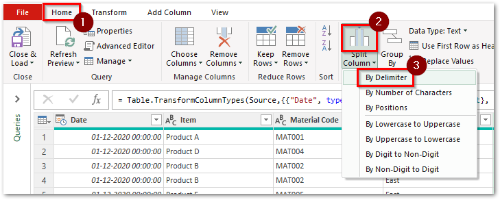
- Now, go to ‘Home’ tab > ‘Transform’ group > ‘Split Column’ > ‘By Delimiter’.
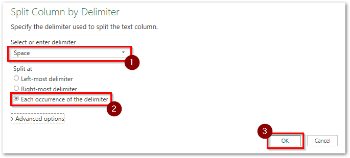
- In the ‘Split Column by Delimiter’ dialog box, select delimiter as ‘Space’. Then, select the ‘Split At’ radio button as – ‘Each occurrence of the delimiter’ and click OK, as shown below:
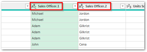
- As a result, you would see that the excel splits the full name into two new columns, one showing the first name and the other containing surname.
- Change the column header name for these two new column by double clicking on it individually.
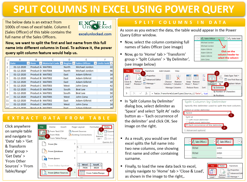
- Now, we are good to reload this table back to excel. Simply, navigate to Home tab > Close & Load as shown below:

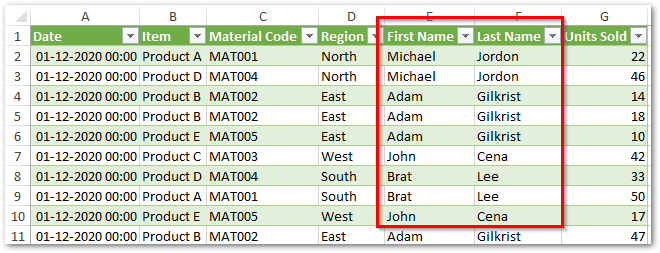
As a result, excel would add a new worksheet to the workbook and add this transformed table to it.
What If There is A Change in Source Table
In addition to what we saw in the above section, the power query feature has an added advantage of quick incorporation of changes.
Suppose, new rows of data are added to the table or there are changes in existing data. You can incorporate these changes immediately in the new table, just by a simple refresh activity.
Let me take one example to make you understand this better.
Suppose I add new rows of data in the original data like this:
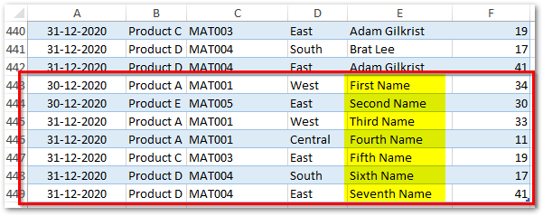
To get the changed data in the new table, right-click anywhere on the new table and choose the option – ‘Refresh’.
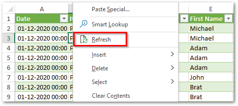
As a result, excel would instantly get the new rows of data to the new table, like this:

Surprised !! Do you know how did this happen? Below is the answer for the same.
While you were splitting the columns in the power query window, excel records it and stores it. Similarly, when you changed the column headers’ name, again the power query editor window recorded it and stored it.
You can see all the recorded step in the ‘Applied Steps’ section of ‘Query Settings’ pane (Power Query Editor Window), as shown below:
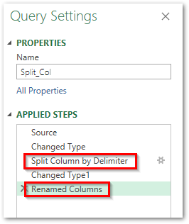
At the time of refresh of the table, the power query re-runs all of these steps and gets the updated data.
In our case, the following steps are performed in sequence – It gets data from the source table, changes the data type, splits column by delimiter, again changes the data type of these new columns, and finally renames the column header.
