Have you ever wondered how to sum the values in the same cell of multiple worksheets? One way is to click on the cell where you want the summation and then select the cells to sum one by one. However, this method is quite a tedious and time-consuming way and is therefore not recommended. You would be happy to know that, without manually adding the values you can even get the sum of values in the same cell of multiple worksheets.
Before directly jumping into the formula let us get our sample data ready.
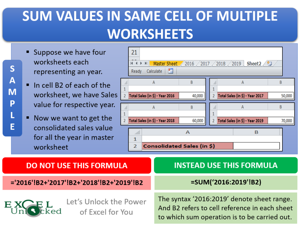
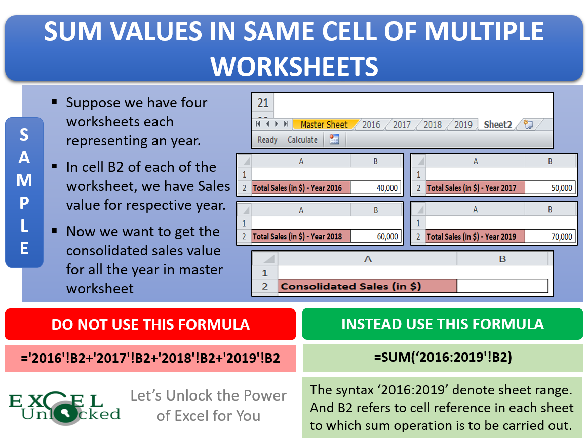
Suppose you have four worksheets (each worksheet representing a year). Cell B2 in each of the four worksheets contains sales value for that particular year.

2016 Sales Value in the worksheet named 2016

2017 Sales Value in the worksheet named 2017

2018 Sales Value in the worksheet named 2018

2019 Sales Value in the worksheet named 2019

In the master worksheet, you want to have the calculated summation of the sales in each year i.e.total sales from 2016 to 2019.

One of the methods is to select the cell where you want to insert the sum and then give reference to the cell B2 from the year worksheets.
Your formula, in this case, would look like as under:
=’2016′!B2+’2017′!B2+’2018′!B2+’2019′!B2

As a result of the above formula, you would get the resultant value as 2,20,000.

However, it would be quite a tedious way to find the sum in a situation where there are hundreds of worksheets and you want to have a total of cell B2 in the master worksheet by giving reference to all the hundred worksheets.
To mitigate this limitation, we can use the sum formula in a different way, which will give you the required result within few seconds.
Sum Values in Same Cell of Multiple Worksheets
To sum the values in same cell of multiple worksheets, enter the following formula in cell B2 of the master worksheet.
=SUM(‘2016:2019′!B2)

As soon as you press enter you would notice that the excel gives the summation result of the cell B2 of each of the worksheets and put it in the cell B2 of the Master Sheet like the way shown in the screenshot below:

Let us now understand each of the components of this formula.

Explanation of the Formula
The =SUM() formula would return the aggregate or summation of the values based on the attribute entered.
The syntax ‘2016:2019’ denotes the sheet range to which you are referring. The year 2016 in our case is the start (first) worksheet name and 2019 is the end (last) worksheet name. The colon “:” between the start worksheet and the end worksheet indicates the range. It means Excel will consider all the worksheets that come in between the first and the last worksheet (included the extremes).
The next one is B2. This is the cell reference for which you want to have the summation operation done.
Both the above attributes (Year range and the cell reference B2) are separated by an exclamation mark (!).
This functionality is not limited to just the summation operation. This even works for: SUM, AVERAGE, AVERAGEA, PRODUCT, COUNT, COUNTA, MAX, MAXA, MIN, MINA, etc.
The Drawback of this Formula
This formula will not work in the case where you insert any row or the column in the Excel worksheet.
It means that this formula would also not move along with the row or column.
This brings us to the end of this blog.

