How to Split Cell Diagonally in Excel

Have you ever wondered how to split a cell diagonally in Excel? By split cell, it means, drawing a line from the bottom left corner of a cell to the top-right corner or from the top-left to the bottom-right corner. In this blog, we would learn multiple interesting ways by which we can split the cells diagonally in Excel.

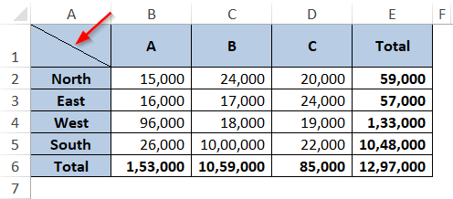
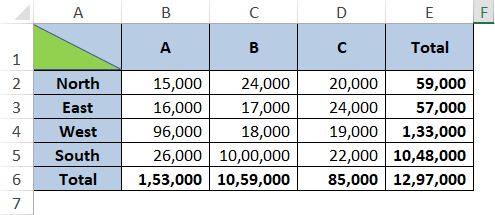
Below is the screenshot of how the split cell would look like:

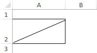
Use of Split Cell in Excel

You might be wondering, how would this type of diagonally split cell help you? This would be a very handy tool when you want to create a table with rows and column heading. Below is an example table. You can see the top-left cell (A1) has been split diagonally to represent what does the row headings and column headings refer to.

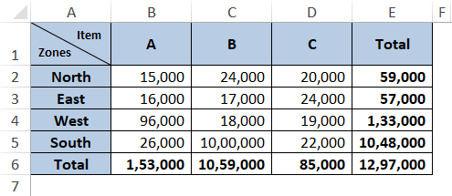
Multiple Methods to Split Cell in Excel

Now, when we are clear with the purpose of the split cell, let us now get an insight into different methods using which we can cut a cell in Excel diagonally.

1. Using ‘Border’ Format
2. By Inserting ‘Line’ Shape in Excel
3. By Inserting a ‘Right Angle’ shape

In the end, we would also learn how to insert the texts on either side of the diagonal line. Just like we have entered ‘Zones’ and ‘Items’ text in cell A1 on the left and right side of the diagonal line.

Let us now begin with each of these methods.

Split Cell in Excel – Using ‘Border’ Cell Format

By default, Excel has provided numerous in-built cell formats that are used to format numbers, fonts, borders, cell fill, etc.

One of the inbuilt cell formats is the ‘Border’ format. It is used to insert and color the cell border in Excel.

We would use this feature to insert cut a cell diagonally in Excel. Follow the below steps:

Select the cell, where you want to insert the diagonal line (I have selected cell A1 – the top-left cell of my excel table).

Now, press Ctrl + 1 on your keyboard to open the ‘Format Cells’ dialog box and go to the ‘Border’ tab as highlighted in the screenshot below:

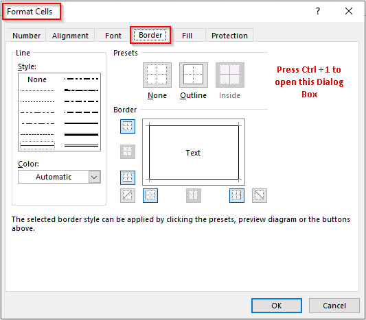
With, this tab, you can perform all the insert border to cell(s), change the color of the cell border, and even the border style to dotted or dash, etc.

Under the ‘Border’ section, you would find two buttons. These buttons insert the diagonal line across the cell corner to split them.

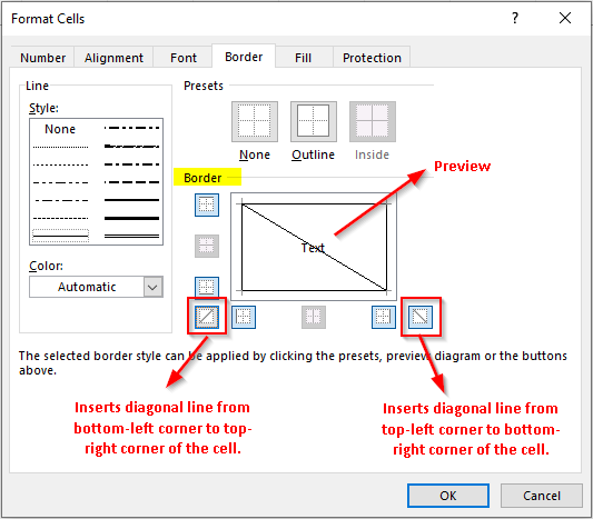
Since my data table has column headings moving towards right and row heading moving downwards, I would prefer to select the button which inserts diagonal line from the top-left corner to the bottom right corner of the cell.

Click OK, after you complete the selection and the excel cuts the cell diagonally as shown in the screenshot below:

By Inserting ‘Line’ Shape in Cell

You can even insert a line shape in the cell to split the cell in Excel. Follow the below steps:

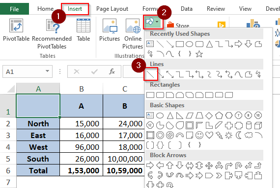
Go to the ‘Insert’ tab and under the group ‘Illustrations’, click on the shapes button. Under the drop-down list of shapes, click on the ‘Line’ shape as highlighted in the screenshot below:

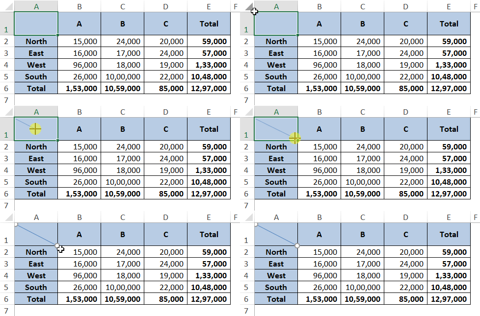
As a result, the mouse cursor would change to a ‘Plus’ symbol like below:

Take your mouse cursor to the top-left corner of cell A1, and left-click on your mouse and drag towards the bottom-right corner as demonstrated in the image below:

This brings us to the end of the second method to insert a diagonal line in a cell.

By Inserting ‘Right-Angle’ Shape

When you use any of the above methods, on drawback is that you cannot give different colors to the two halves (triangles) in the cell A1. The fill color can be given to the entire cell A1 and it fills both the sides of the diagonal line.

However, if you wish to give different colors to the two halves in cell A1, this method best suites.

Follow the below steps:

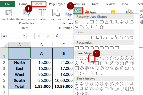
Go to the ‘Insert’ tab and under the group ‘Illustrations’, click on the shapes button. Under the drop-down list of shapes, click on the ‘Right-Angle’ shape as highlighted in the screenshot below:

Similar to the above method left click and drag and drop the shape inside the cell A1. As demonstrated in the image below).

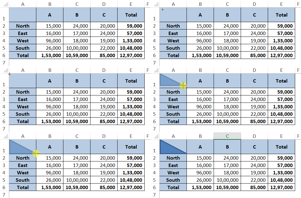
Now, you can easily format this ‘Right Angle’ shape and give different color to it like below:

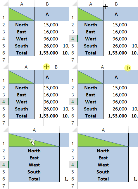
The most amazing thing about all the above methods is that when you can the column width of the cell, the shapes, and the diagonal borders also adjusts itself. Below screenshot explains this:

Inserting Text in Split Cells

Now, we would learn how to insert the texts on either side of the diagonal line. One of the methods is to insert a text box and place it on the relevant side of the diagonal line.

To insert a text box, go to the ‘Insert’ tab, and click on the button ‘Text Box’ under the group ‘Text’ as highlighted in the screenshot below:

The mouse cursor would change to a vertical line like a symbol.

Click on the location where you want to type and adjust the font size accordingly.

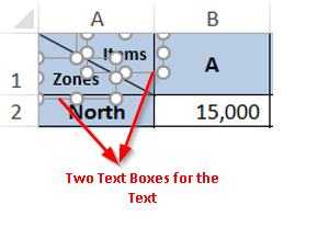
Another method to insert the text on either side of the diagonal lines is entering the texts in the cell A1 itself (without inserting text box).

Follow the below steps:

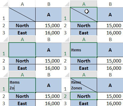
Enter the first heading text “Items” and then press Alt + Enter to insert a line break and move to the next line in the same cell. In the next line, enter the second heading text “Zones”.

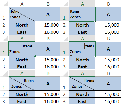
Now, place your cursor on the left side of the text ‘Items’ and insert the required spaces. Similarly, adjust the word ‘Zones’.

Note that this method would not be useful when you have split the cell using the ‘Right-Angle’ shape. In this case, you need to use the ‘Text Box’ to write the rows/column headings.

This brings us to the end of this blog, share your views and comments in the comment section below.