Excel TRANSPOSE Function – Rotate Columns to Rows

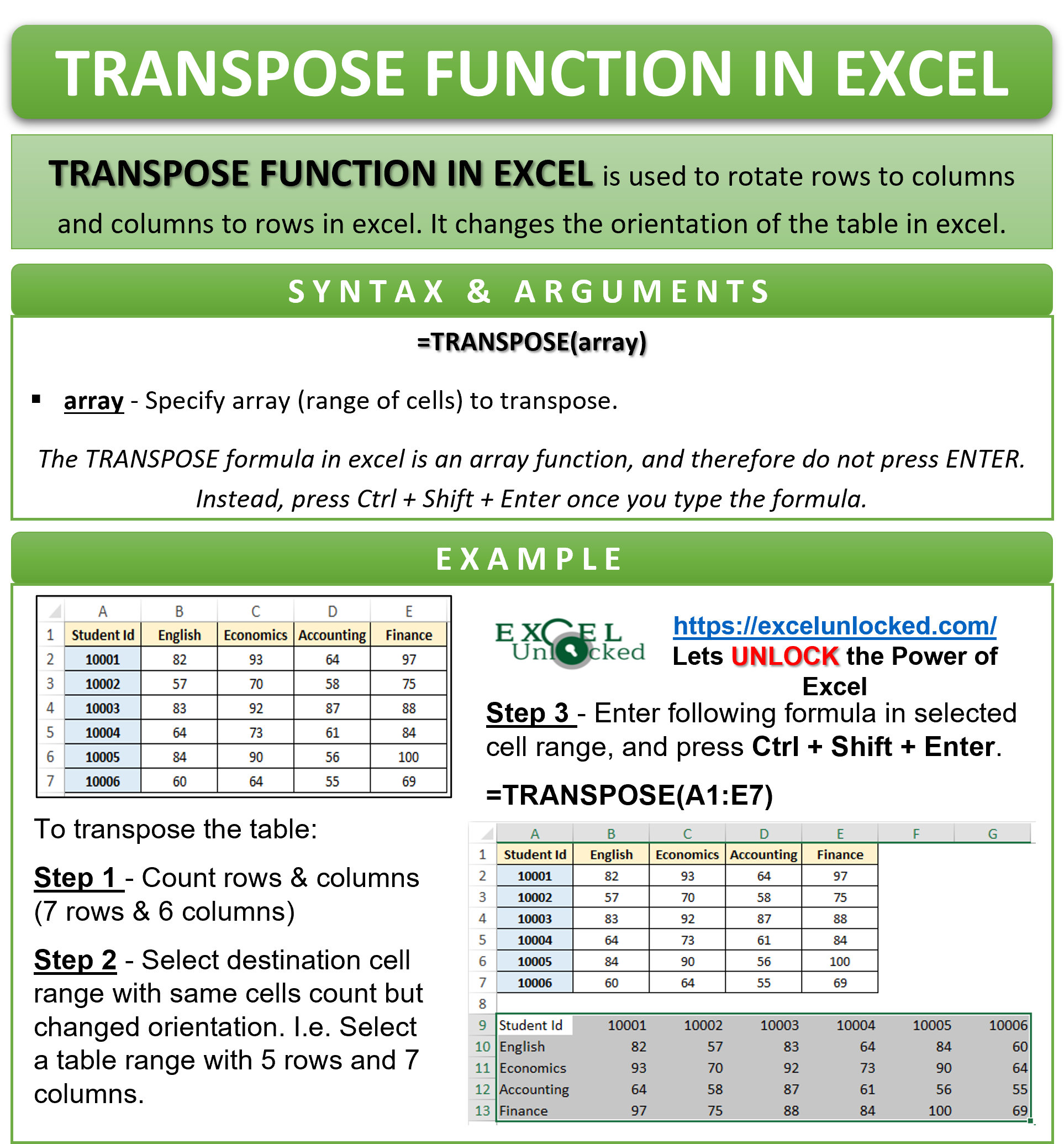
Many a time, you may wish to change the orientation of data (i.e convert horizontal data to vertical or vertical data to horizontal) in Excel. When the data is large, converting the column to row and vice versa manually is not a good option. To achieve this quickly, excel has come up with the functionality of transpose data in excel. There are multiple ways to transpose data in excel. In this tutorial, we would learn the formula method to transpose data in excel, called the TRANSPOSE function in Excel.

Here we go 😎

When To Use TRANSPOSE Excel Function

The TRANSPOSE formula in excel is used to change the layout of the data by rotating columns to rows and rows to columns. This function converts row to column and vice versa.

This function belongs to the Reference formula group in excel.

Syntax and Argument

=TRANSPOSE(array)

This function just has one argument viz. array.

• array – In this argument, specify the range of cells that you wish to transpose.

It is important to note that the Excel TRANSPOSE formula is an array function. Consequently, you must press Ctrl + Shift + Enter to return the array result.

Example of TRANSPOSE Function in Excel

The TRANSPOSE function belongs to the array function. Therefore, it will not work by simply using the formula as we do for other excel functions in general.

Let us now learn how to use the TRANSPOSE excel formula by taking an example, and what’s so special about it.

The below image contains the marks obtained by 6 students in 4 subjects.

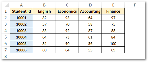
Now, suppose you want to change the orientation of this data table in excel using a formula i.e. rotate column to row and rotate row to column.

To achieve this simply follow the below steps without any mistake.

Step 1 – Count Rows and Columns in Original Table

To start with, firstly count the number of rows and columns in the source data table. In our example, there are 7 rows and 5 columns.

Keep these row and column counts in your mind, and let’s now move to the next step.

Step 2 – Select Destination Cells with Same Cells Count, but Changed Orientation

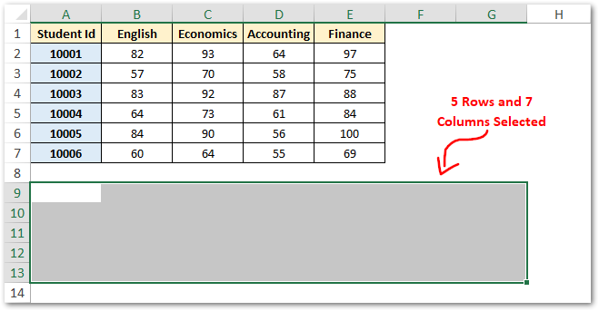
In step number 2, you need to select the blank cells where you want to place the transposed table. However, the trick is that,

• The count of rows in selected cells must be equal to the count of columns in the original table (i.e. 5); and

• The count of columns in selected cells must be equal to the count of rows in the original table (i.e. 7).

That is, select a table range with 5 rows and 7 columns.

Step 3 – Using TRANSPOSE Array Formula

This is the final step to transpose the data table in excel.

Simply, type the following formula, but do not press ENTER key.

=TRANSPOSE(A1:E7)

Your excel sheet would look like this after the above step:

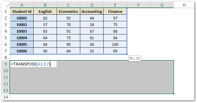
As you can see from the above data, cell A9 is still in edit mode as I have not pressed ENTER key yet.

Finally, press Ctrl + Shift + Enter key combination on your keyboard to return the array formula result. With this, the formula gets applied to all the cells in the selected cell range A1:E7.

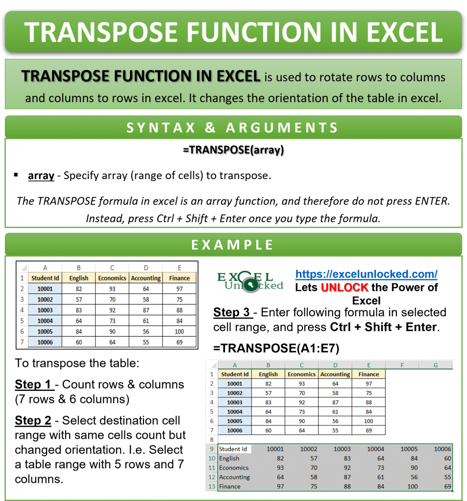
Here you go 😉 The original table gets transposed successfully.

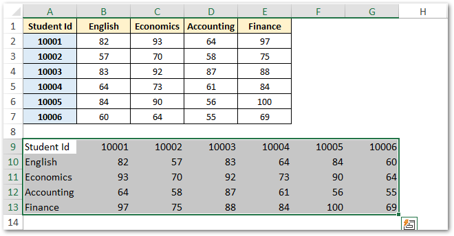
Do Not Miss These Points

Although using an array function was easy over here, however, some points may be confusing to inexperienced users of the Excel TRANSPOSE function.

• As soon as you press Ctrl + Shift + Enter on your keyboard, the excel would add curly brackets around the formula in the formula bar. It simply denotes that the formula is an array formula.
  
  Do not ever try to add the curly brackets manually, as it wont work.

• You cannot edit only a part of an array formula like TRANSPOSE. To change the TRANSPOSE formula, select the entire range (in our example, A9:G13), then make required changes to your formula and finally press Ctrl + Shift + Enter.

• Similarly, to delete the transpose formula, firstly select the entire range of cells (A9:G13) and then simply press ‘Delete’ key on your keyboard. This will remove the transpose formula from the selected cell range.

• When you transpose the table data using the TRANSPOSE formula learned above, the there exists a link between the two tables. This means that any change in the original dataset table will reflect in the transposed table. To remove connection between original table and transposed table, simply follow this procedure:
  • Copy the entire range of transposed table (A9:G13)
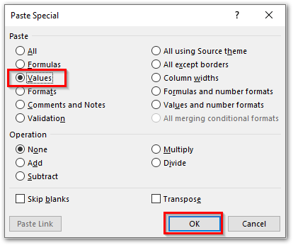
  • Use Ctrl + Alt + V to open ‘Paste Special’ dialog box
  • Select radio button ‘Values’ and press OK.

Apart from using the TRANSPOSE excel formula, you may also try some other ways and methods to transpose data in excel.

Thank you for reading 🙂