TYPE Function in Excel – Get Data Type

The TYPE Function in Excel is a vital Information Function. It can perform the working of ISNUMBER, ISTEXT, ISLOGICAL, and ISERROR in one go and also has other abilities.

When to Use TYPE Function?

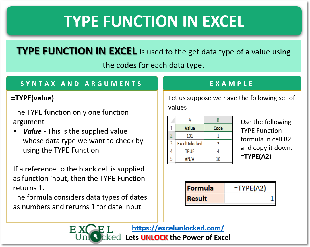
The TYPE Function in Excel is used to know the data type of a supplied value. It is just that, any value in Excel would either be a Number, Text, Logical Value, Error Value or an Array of Values.

The TYPE Function returns the data type with a certain code assigned to each data type. Following are the codes for a set of different data types.

Data Type (Supplied Value)	Code (Function Result)
Number	1
Text	2
Logical Value	4
Error Value	16
Array	64

Syntax and Arguments

=TYPE(value)

The TYPE Function needs to be supplied with only one function argument.

• value – This is the supplied value whose data type we want to check by using the TYPE Function

Important Points About TYPE Function

Here we have some important points to remember about the TYPE Function.

• The TYPE Function can be used in Excel 2000 and later versions of Excel.
• The function returns 16 if the input is an error value.
• If we supply a formula as the TYPE Function argument, the code is returned based on the data type of the result of the input formula.
• The formula considers data types of dates as numbers and returns 1 for date input.
• If a reference to the blank cell is supplied as function input, then the TYPE Function returns 1.

Example for TYPE Function Formula

In this section of the blog, we are going to implement the TYPE Function with the help of some examples.

Example 1 – Basic Example for TYPE Formula

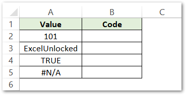
Let us suppose we have the following values in the range A2:A5.

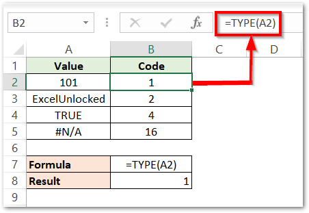
Use the following TYPE Function formula in cell B2 and copy it down the range B2:B5.

=TYPE(A2)

As a result, we get the codes in the range B2:B5.

Explanation – We have supplied cell A2 containing a numerical value 101 as the TYPE Function input. Since this is a numerical value, the formula returns 1 meaning for the numerical data type of value in cell A2.

Similarly, we get 2,4 and 16 because the value in cells A3, A4 and A5 is a text string, Logical Value and an Error Value respectively.

Example 2 – Other TYPE Function Formulas

Here, we have other examples for the TYPE Function formula.

=TYPE(10-10-2002)

The data type of Dates is also a numerical value, which is why the TYPE formula returns 1.

Now we would input a formula to see the data type of formula result.

=TYPE(RANDBETWEEN(20,10))

The RANDBETWEEN formula returns a #NUM! error when the bottom value is greater than the top value which is true for this formula. The TYPE Function gets a #NUM! as input and we get 16 as result.

This brings us to the end of the blog.

Thank you for reading.