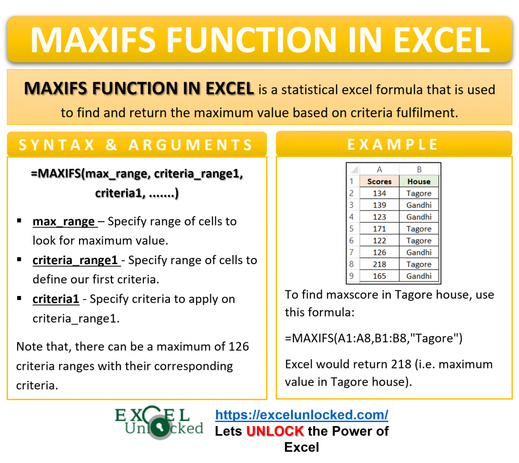
In one of the previous tutorials, we learned the MAX function and MAXA function to find the maximum value without any criteria check. Let us now learn another excel function called the MAXIFS function in excel. The MAXIFS formula is used to find the maximum value based on the specified criteria or criterias.
Here we go 😎
When to Use Excel MAXIFS Function
The Excel MAXIFS formula finds the maximum numerical value from the specified range of cells based on the criteria. This function forms part of the basic statistical function.
With the use of the MAX function in excel, we could find the maximum marks for the entire class. But by using MAXIFS, we can look for the maximum score for section A or Tagore house students.
Syntax and Arguments
=MAXIFS(max_range,criteria_range1,criteria1,…….)
The below points explain the function arguments of the MAXIFS formula in excel
- max_range – In this argument, specify the range of cells to look for the maximum value.
- criteria_range1 – In this argument, specify the range of cells to define our first criteria.
- criteria1 – In this argument, specify the criteria to apply on the criteria_range1. It can be a number, text string or an expression having wild cards characters or logical operators.
There can be a maximum of 126 criteria ranges with their corresponding criteria. It is important to specify at least one criteria in the MAXIFS formula. Therefore, the remaining 125 criteria are optional arguments.
Points to Remember About MAXIFS Excel Function
You should remember the following points about the MAXIFS formula before its actual usage.
- The function uses AND logic for multiple criteras. It will return the maximum value that satisfies all the criterias. (Explained in Ex. 2)
- We can use logical operators like >, <, <>, = in the MAXIFS criteria.
- Use Wild Cards ( * or ? ) when you have a fussy guess for the matching ctiteria with the criteria range.
- MAXIFS function is not case sensitive.
- If you take text strings in max_range, then it would return a zero.
- max_range and criteria_range should have the same number of elements.
- Criteria in syntax
- Strings and dates will be in double quotes while numbers and cell refrences should not, when used on their own
- When we are using logical operator in the criteria, the whole expression will be closed in double quotes like “<10” whereas function and cell refrence must be concatenated using an ampersand like this “>”&A2 or “<“&TODAY().
Examples to Learn MAXIFS Function in Excel
This section of the blog will explain to you some of the most practical examples for the Excel MAXIFS formula.
Ex. 1 – Passing One Criteria in MAXIFS Function
Below are the scores of students in the inter-house badminton competition.
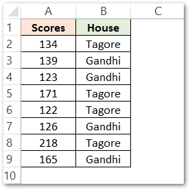
Enter the following MAXIFS formula to find the maximum score in the students of Tagore House.
=MAXIFS(A1:A8,B1:B8,"Tagore")
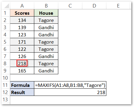
As a result, the function will return 218.
Explanation – In the above example, we have specified the criteria1 as “Tagore”. The Highlighted rows are the records for students of Tagore house. There are four students who participated from Tagore house and their corresponding scores are 134, 171, 122, and 218. The MAXIFS function applied the criteria and then returned the maximum value from these four scores. The maximum score in Tagore house resulted out to be 218.
Ex. 2 – Passing Multiple Criteria to MAXIFS Function in Excel
The MAXIFS function works on the AND logic when multiple criteria are passed to it.
In this example, we will find the maximum score of the student from section A having Tagore house.
Below is the data containing scores, house, and section information about the student.
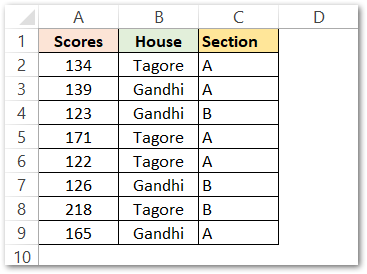
Enter the following MAXIFS formula to find the maximum score from section A having Tagore house.
=MAXIFS(A2:A9,B2:B9,"Tagore",C2:C9,"A")
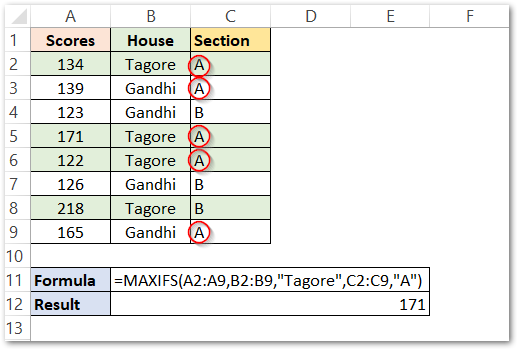
The result of the above formula is 171.
Explanation- The first criteria is set to “Tagore” for the criteria_range B2:B9. The records that satisfy this criterion are 134, 171, 122, and 218. Whereas the second criteria is set to “A” for the critera_range C2:C9. The records that satisfy criteria 2 are highlighted in red circles. Their corresponding scores are 134, 139, 171, 122, and 165. The MAXIFS formula will look for the maximum value in the range of cells that satisfies both of the conditions simultaneously 134, 171, and 122. Therefore, the final result of the formula is 171 (highest of all the three).
Ex. 3 – Passing Logical Operators with Number in MAXIFS Formula
In this example, we would pass an expression containing a logical operator in the MAXIFS function in excel.
Below are the sales of the company and the corresponding age of the employees. We will find the maximum sale of the employee whose age is more than 25 (i.e. 25+).
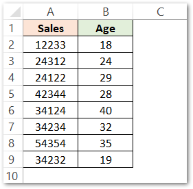
Use the following MAXIFS formula to find the maximum sales done by the employees having 25 plus age.
=MAXIFS(A2:A9,B2:B9,">25")
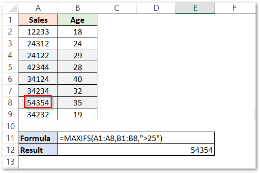
As a result, the formula output comes out to 54354.
Explanation – The criteria is the expression “>25”. The records corresponding to this condition (age more than 25) are highlighted. The maximum value of sales from 24122, 42344, 34124, 34234, 54354, and 34232 is 54354.
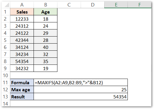
Note – We can also use cell reference with the logical operator, the only difference is syntax. We do not put cell references in inverted commas when used with the logical operator. Instead, the cell reference is concatenated by the logical operator by using an ampersand or CONCATENATE function.
EX. 4 – Using Wildcard characters in MAXIFS Formula of Excel
Whenever we have a fussy guess about what we looking for, wild card characters come into use. Following are the wild cards in excel.
- ? – Use it when you have no clue of single character.
- * – Use it for a sequence of characters that are unknown.
Check our special blog on Wildcard Characters in Excel to learn more about excel fussy characters.
The below image contains the order IDs and the corresponding product quantity against the order ID. The company has two teams named Katmandu Products and Manipur Products. The order IDs ends with /KP and /MP respectively.
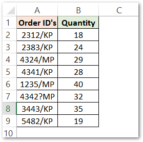
Let us now use the MAXIFS formula to find the bulk order at Katmandu Products.
=MAXIFS(B2:B9,A2:A9,"*KP")
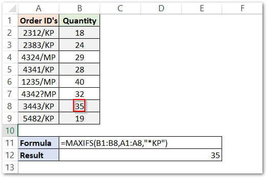
As a result, the formula will return the maximum value as 35.
Explanation – The criteria is set to “*KP” which means that the formula will find all the records which end with the text “KP”. The highlighted records are the records that satisfy this criterion. Finally, the maximum value of quantity for Katmandu Products is 35.
With this, we have reached the end of this tutorial on MAXIFS function in excel.
Thank you for reading 🙂

