In our previous blog, we learned the IRR Function of Excel. In Finance, whenever we want to get the IRR when consecutive cash flows have a difference of 1 complete year between them, IRR Function is used. XIRR function in Excel works like IRR function, gives us an internal rate of return with a slight difference of an additional input parameter. Let us go to the depth.
Here we go 😎
When to Use XIRR Function of Excel
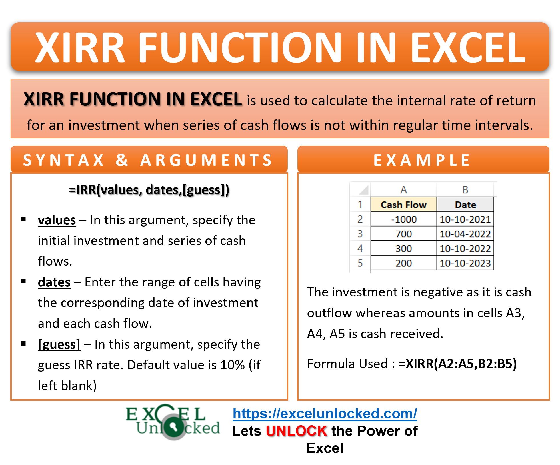
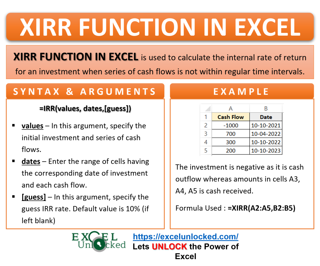
The XIRR Function of Excel gives the internal rate of return for a project when the series of cash flows is not within regular time intervals. We need to mention the dates for each cash flow whether it is money received or deducted.
The XIRR Function comes under the category of Financial functions of Excel.
Syntax and Arguments
=XIRR(values,dates,[guess])
The following points contain the information required for the XIRR Function arguments.
- values – Values is the range of cells containing an initial investment or amount with a consecutive series of cash flows.
- dates – Dates is the range of cells having the corresponding date of investment and each cash flow. The consecutive date must be greater than the prior.
- guess – This is an optional XIRR function argument. IRR can have two values for same project. guess is a rough estimation for resultant IRR.
Points to Remember About XIRR Function
The following points contain the basic information required to use the XIRR function correctly.
- XIRR returns the discount rate that makes the XNPV = 0. XNPV is the Net present value of cash flow for the irregular intervals.
- The default value for guess is 10% or 0.1.
- Dates should be in the correct format. It can be a range of cells or the result of other formulas.
- The values function argument requires at least one positive and one negative value.
- value and dates arrays must be of the same length.
- There is a maximum of 100 iterations.
- Every date in Excel has its own numerical value. For instance, 1 Jan 1900 is 1, 2 Jan 1900 is 2. Dates earlier than 1 Jan 1900 are invalid dates in Excel and make the function return a #VALUE! error.
Examples for XIRR Function of Excel
In this section of the blog, there are some practical examples that will make you go through the usage of the XIRR function of Excel.
Ex.1 – Simplest Example for XIRR Function
In this example, let us say there is an investment of $1000 on 10 Oct 2021. This investment will give an earning of $700, $300 and $200 after 6 months, 1 year and 2 years respectively. The investor wants to know the IRR for this project.
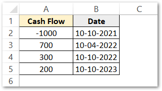
The investment is negative as it is cash outflow whereas the rest of the money in cells A3, A4, A5 is cash received after investing money so it is positive.
Use this XIRR Formula to get the Internal Rate of Return for the above project.
=XIRR(A2:A5,B2:B5)
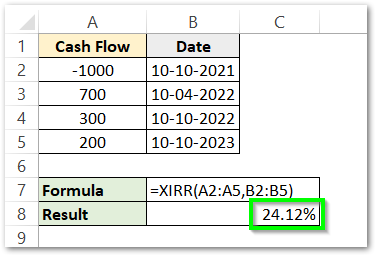
As a result, the function has returned 24.12 % as the IRR.
Explanation – We have passed the range A2:A5 as the values function argument for the XIRR function. The range contained cash flows for the coming dates. B2:B5 has the dates for each cash flow passed to the function argument. A2 contains a negative value of cash outflow. The XIRR Function has returned the IRR or discount percentage for the project that makes its Net Present Value or XIRR = 0.
Let us see how.
Verifying XIRR Function results
In this section, we will manually verify the IRR result given by the XIRR Formula in the first example. To understand the concept, we need to first go through these points.
- Money loses its value when it travels from present to future. In other words, 1000 rs today would never be worth the same as 1000 rs after 10 years.
- The future cash flows are discounted to get their present value. The rate is known as discount rate.
- XNPV is the Net Present Value of Cash flows when they are not in regular intervals of time.
- Internal Rate of Return is that value of discount percentage that makes the XNPV = 0. We use XIRR for irregular cashflows and IRR for regular cashflows.
The formula to calculate the present value of money from the future value is
PV=FV/(1+IRR%)^t
PV= Present Value
FV= Future Value
IRR= Discount %
t= Time
We have added a column for a time in each cash flow. The time represents the number of years between the initial investment and the corresponding cash inflow. Use this formula to get the PV for each cash flow.
=A2/(1+$F$4)^C2
where A2 has the FV. F4 is IRR% and C2 is time.

As a result, the formula has returned the PV for cash flows. We have used the Excel fill handle tool to copy the formula for the rest of the cashflows.
The IRR value used in the above formula was calculated in the first example by using the XIRR Function.
Use this SUM formula to get the Net Present Value.
=SUM(D2:D5)
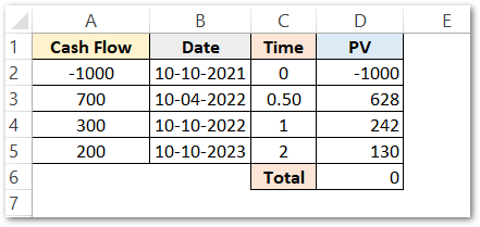
The sum of NPV comes out to be zero when we took the IRR = 0.24
This verifies our result in example 1.
Ex.2 – Using IF Function to Pass Dates in XIRR Function
In this example, let us say there are two projects with initial investments of $1200 and $1450. Following are the cash flows received after the investment for Project A and B. Both of the projects were signed on 10 Oct 2020.
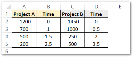
Time is the time in years from the initial investment for each cash inflow. Use the following XIRR Formula merged with IF and CHOOSE Function of Excel.
=XIRR(A2:A5,IF(1,CHOOSE({1,2,3,4},"10-10-2020","10-10-2021","10-4-2022","10-4-2023"),""))=XIRR(C2:C5,IF(1,CHOOSE({1,2,3,4},"10-10-2020","10-4-2021","10-10-2022","10-4-2024"),""))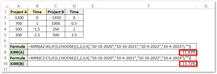
As a result, the function has returned the Internal rate of return for both projects as 11.83% and 13.72%.
Explanation – We have passed two arguments in the XIRR function. The values function argument has the range A2:A5 which is the cash flows for project A. The initial investment is negative for both of the projects. We have used the result of the IF formula as the dates function argument of the XIRR formula. However, you can see the stepwise explanation for the dates function argument as follows
Step Wise Explanation
- The IF function has three arguments. First is the condition, which is 1. Condition 1 means a logical TRUE and will always make the condition TRUE in this case.
- The second IF function argument contains the formula result if the condition is TRUE. CHOOSE Function contains an array of indexes as {1,2,3,4} which would return the four values that contain the dates for cash flows. The Dates are always enclosed in double-quotes.
- As the condition is TRUE, the IF function returns an array for dates XIRR function argument. This would be “10-10-2020″,”10-10-2021″,”10-4-2022″,”10-4-2023”
- The third IF function argument (“”) did not implement as it implements only if the condition is FALSE.
The XIRR Function calculates the IRR for both of the projects by the values and dates function argument. Project B is more profitable than Project A because of more IRR %.
Thank you for reading 😉
RELATED POSTS
- Excel RATE Function – Calculating Interest Rate for Specified Period
- NPER Function in Excel – Calculating Number of Periods
- FV Function of Excel – Find Future Value of Investment
- Excel XNPV Function – NPV With Irregular Cash Flows
- Excel PV Function – Calculate Present Value PV in Excel
- ISPMT Function of Excel – Interest Amount Keeping the Principal Constant

