Make Your Own Chart Template in Excel

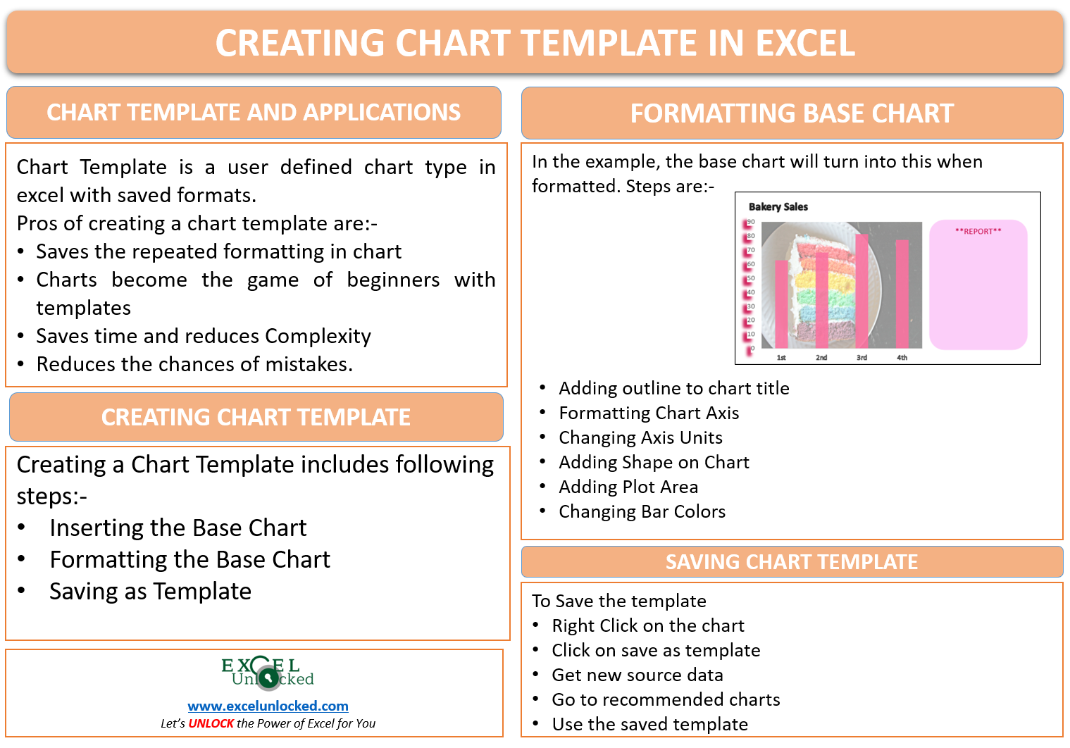
Chart Template in Excel is a time saver hack. Do you have to deal with charts in excel and have a fixed chart type, formatting, plot area, chart area and so much more that you want to repeatedly use in your projects? Then you are in right place. Chart templates can be customized and saved to make those formats saved in the form of a chart template.

Let us see how 😎

Why do I need a Chart Template

Charts in Excel have so much updated and evolved, when a person looks at these charts it seems as if these charts need some professional person to get the things at right place. Chart Template in Excel makes the job a lot easier as they will save all the formats on the charts and the new user would only have to use the template. All the formatting once saved need not be repeated once again by someone who doesn’t have charting techniques.

Creating a Chart Template

Let us say Umesh is a business owner and he wants the employee of his company to make a monthly report. The report contains a chart for weekly sales for each month. The report for all months must be in the same format. Umesh is not sure if the new employee would be able to handle all the chart formatting so he wants to create a chart template in Excel so that the employee doesn’t get mixed as there is no space for mistake.

From here we will move in steps.

Choosing the Data Type

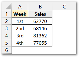
The chart template can be used for the same type of data. In this example, we have the weekly sales that will be represented with the help of a column chart in excel. Below is the data.

Inserting the Base Chart

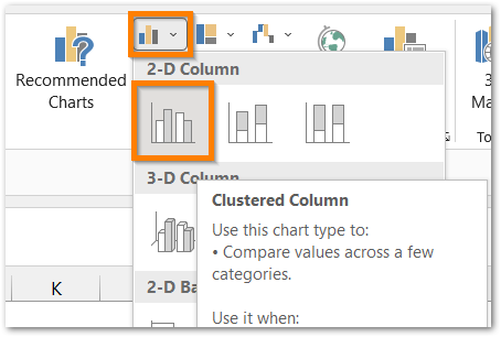
There are so many types of charts in excel including column charts, line charts, pie charts, etc. However, in this example, we would take a column chart. Now select the range A1:B5 and :

• Go to insert tab
• Move cursor to charts group
• select the column chart button

Consequently, you can press alt + F1 to get the default chart type for this type of data.

A column chart inserts in the worksheet and it will act as the base chart for the template.

Apply Chart Formatting

Following is the base chart.

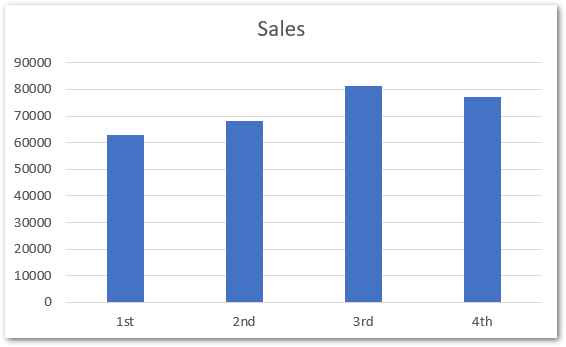
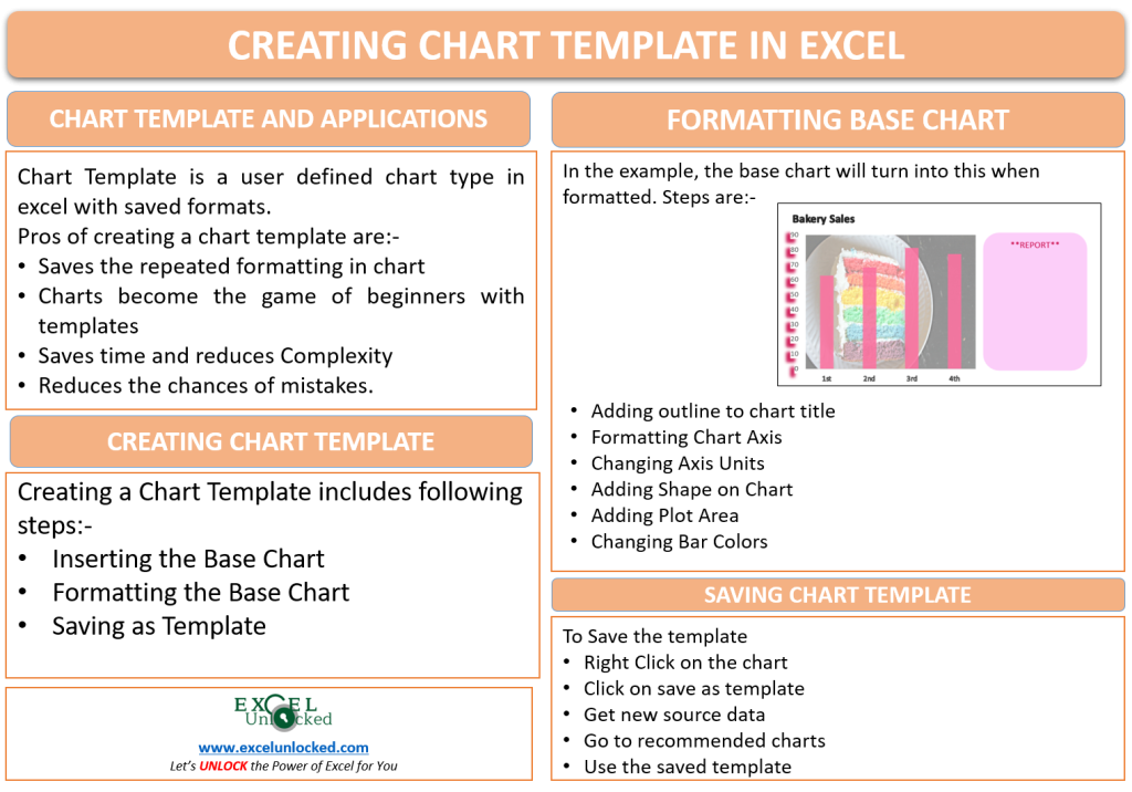
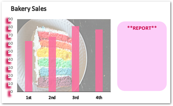
Firstly, We will format this chart and make it look something like this.

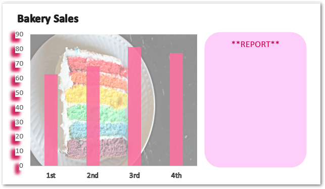
This is going to be the final chart template. The steps to format the base chart to the final chart are:

Step 1 – Adding Outline to Chart Title.

We have changed the chart title to “Bakery Sales”. To make the title cleaner, we have added a black outline around the text. Following are the steps:-

• Select the chart and go to Format Tab.
• Choose Chart Title in the Current Selection group.

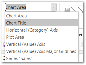
• Click on the button Format Selection.

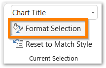
• The Format Chart Title Pane on the left of excel appears. Select text border as black from there.

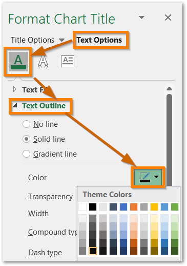
As a result, the outline adds to the text making it bold.

Step 2 – Formatting Chart Axis

Firstly, we will format the horizontal axis. However, we will add an outline as we did to the chart title.

• Select the Chart, In the format tab under the Current Selection Group
• Choose Horizontal Axis now.

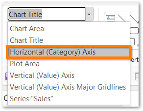
• Repeat the procedure as you did for chart title. Add text outline from Format Axis Pane

Consequently, we will now format the vertical axis in a different format.

• Change the current selection to Vertical Axis and Click on Format Selection Button.

• Set the Shadow color and set the following values to the five sliders or you can adjust them as you wish.

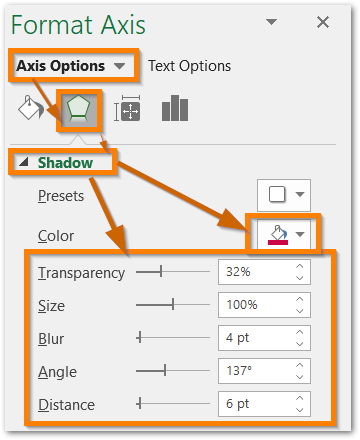
Step 3 – Changing Axis Units

We will now change the axis units for the y-axis and express it in thousands.

• Right Click on the Chart and Change the Current Selection back to Vertical Axis.
• Click on the Format Selection Button.
• In the Format Axis Pane, choose the display units as thousands

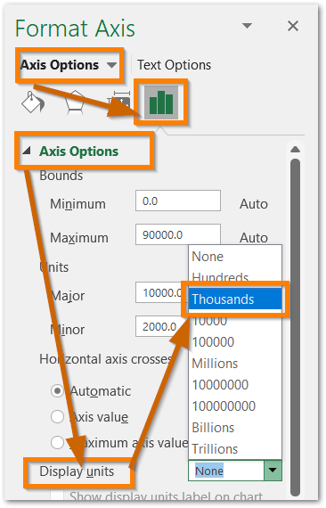
• The vertical chart axis values change to x thounsands.

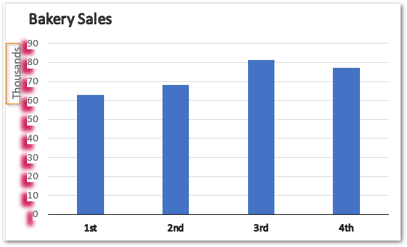
It is your wish to keep the “thousands” as display units on the chart. For now, we are removing it by simply selecting it and pressing the delete key.

Step 4 – Adding Shape on Chart

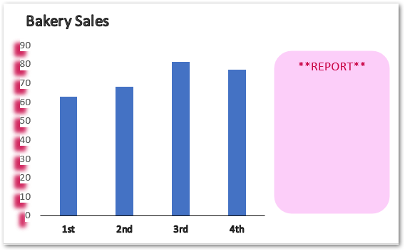
We will now make space for the chart to add shape to it by dragging the plot area. Click on the plot area and you will see the pull handles. Drag the right pull handle towards the left.

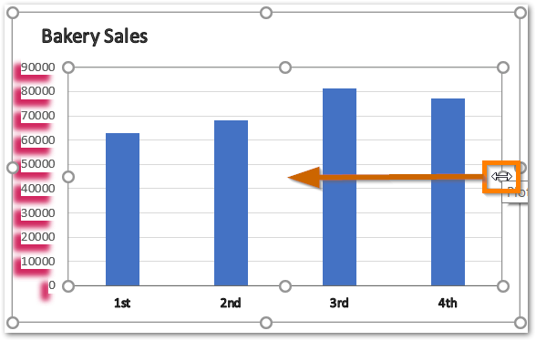
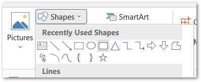
Go to the insert tab and choose the desired shape to put into the chart. Go to the shape format tab and select the shape fill color.

Make sure that the chart is selected when you are inserting the shape. If you did not select the chart before inserting the shape, it will not be saved with chart while saving the template.

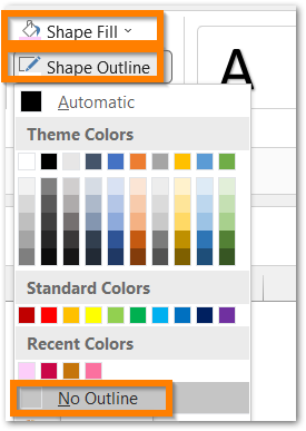
Set the shape boundary to no boundary. Type “**REPORT** in the shape.

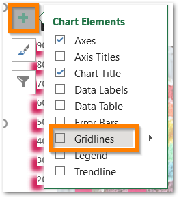
After that, You can remove the grid lines by clicking on the chart + arrow and unchecking the gridlines. You can add or remove other chart elements also.

This is how the chart will look now.

Step 5 – Adding Plot Area

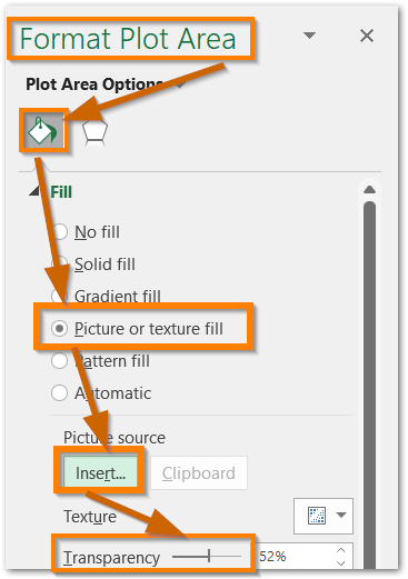
We will now add a background image that matches our business to the plot area. To do that:-

• Click on the chart and select plot area in the current selection (Format Tab)
• Click on Format Selection. The Format Plot area pane will open at the left of the excel window.
• Choose the picture to be inserted and increase its transparency to 50 %.

Step 6 – Changing Bar Colors

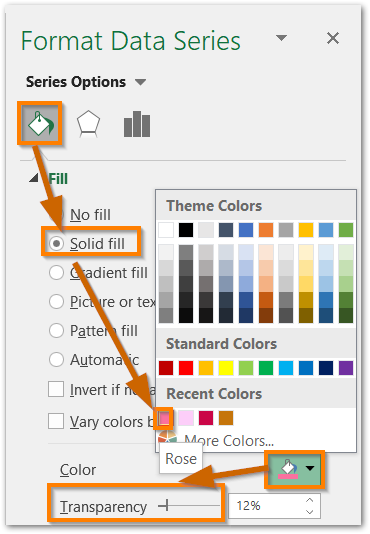
We will now adjust the color of the bars in the column chart.

• Select the chart and go to format chart.
• Choose Series “Sales” in the Current Selection and Click on Format Selection.
• Select the fill color and increase its transparency to 12 %.

Saving the Chart Template

Lastly, we have got our chart formatted, and below is the result.

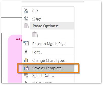
Right Click on this chart and select save as template from the shortcut menu.

The Save Chart Template Dialog box appears. Set the name and click on save. For now, we are saving the chart template with the name “cake”.

Using Chart Template

As we have now saved our chart template. Open a new worksheet and enter the data:-

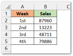
To use the chart template:-

• Select the range A1:B5 and go to insert tab.
• Click on recommended charts button
• The Insert Chart Dialog Box opens. Go to All Charts tab.
• Click on Templates folder in the menu and select the template you saved earlier with the name “cake”.

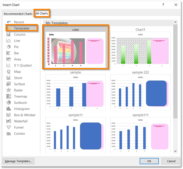
The chart with the saved chart template in excel would be inserted. The only difference is of source data.

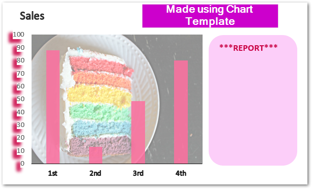
This brings us to the end of the function blog.

Thank you for reading 😉