Custom Error Bars in Excel – Adding and Deleting

In the earlier blog, we learned about the usage and different types of Error Bars in Excel. Custom Error bars are one of a special kind of error bars. In this blog, we will be learning about how the custom Error Bare is created, adding Error Bars only to a specific Data Series, and deleting error bars. So let us start learning.

What are Custom Error Bars?

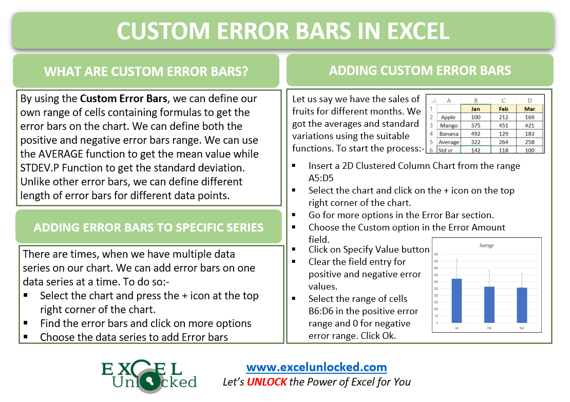
By using the Custom Error Bars in Excel, we can define our range of cells containing formulas to get the error bars on the chart. We can define both the positive and negative Error range. We can use different functions like the AVERAGE Function to get the mean of values while STDEV.P Function to get the value of standard deviation.

Unlike all other Error Bar types, we can define different length error bars for each of the data points by using the range of values.

Example – Adding Custom Error Bars in Excel

Let us suppose we have the sales of different fruits for three months as follows:-

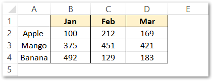
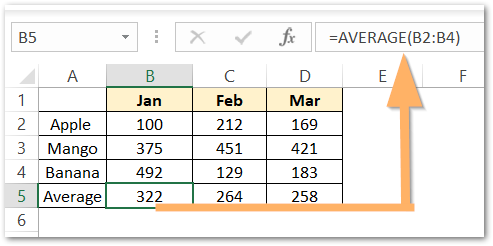
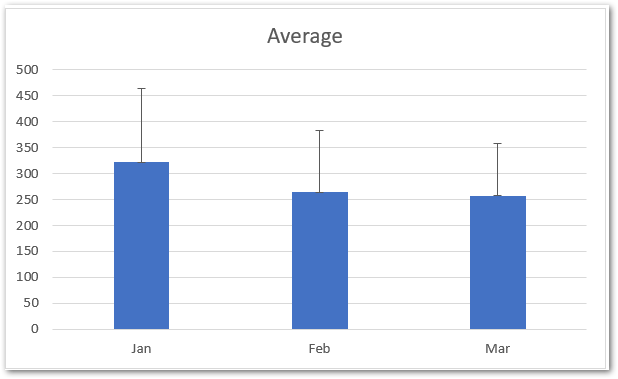
We want to create a column chart representing the average sale of each fruit in a month. So we will use the below-mentioned formula in cell B5 and copy it using the fill handle tool.

=AVERAGE(B2:B4)

This gives us the average sales as follows:-

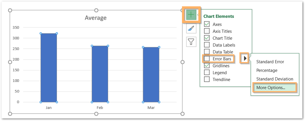
We would now insert a Column Chart from the range A5:D5.

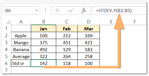
In this chart, we only have one data series representing the average fruit sales. Find the Standard Variation for each data point by using the STDEV.P Function of Excel. Use the following formula in cell A6 and copy it to the right up to cell D6.

=STDEV.P(B2:B5)

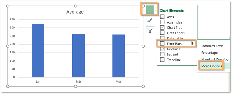
Now click on the + icon on the top right corner of the chart and choose More options for Error Bars.

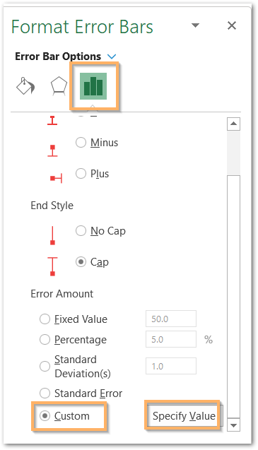
This opens the Format Error Bars pane. Choose the Error Amount as Custom Error and click on the specified value button.

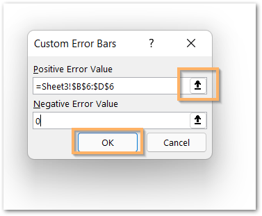
Now clear the contents of both the Positive and Negative Error fields. Select the range B6:D6 for the Positive error value and type 0 as the negative error value ( this removes the negative error bars )and click ok.

This inserts the custom error bars on the chart as follows:-

Adding Data Bars to a Specific Series in Chart

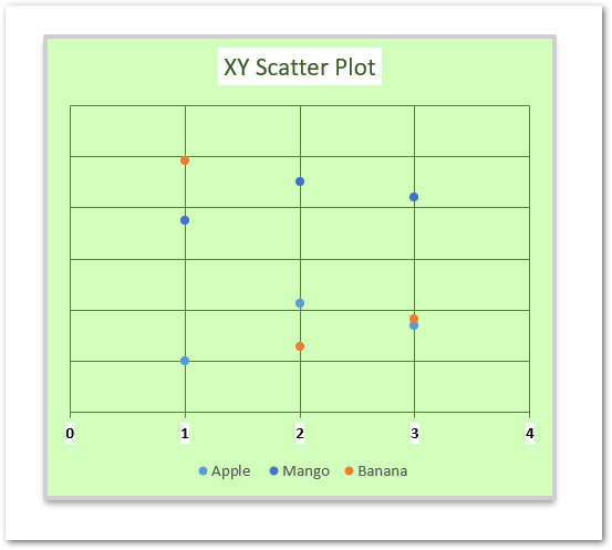
We can have multiple data series in one chart. Let us say we have the following scatter chart:-

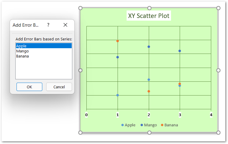
If you go for more options for adding the error bars from the + icon at the top right corner of the chart, a dialog box appears asking for the series you want to add the error bars for.

Deleting the Error Bars

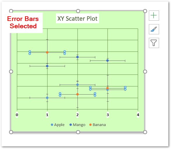
You can delete the error bars by simply unmarking the error bars or by simply selecting them and pressing the delete key.

This brings us to the end of the blog

Thank you for reading.