A Complete Guide on Sparklines in Excel

In our earlier blog, we learned the basics of Sparklines, including the definition, types, and insertion. In this blog, we will be covering the total functionality of Sparklines in Excel.

Grouping and Deleting the Sparklines

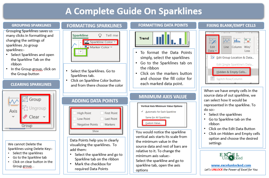
By grouping we mean, to collect the sparklines and let them be in a group so that all the sparklines could be formatted and changed collectively without having the need to separately do changes on each sparkline.

To group/ungroup the sparklines

• Select the sparklines.
• Go to Sparkline Tab on the ribbon
• In the Group column, group your sparklines in case they are ungrouped.

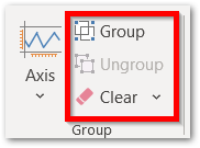
There are three options, from the group/ungroup only one button is clickable as the sparklines could either be grouped or ungrouped at one time. Below is a button to clear the selected sparklines as we cannot delete the sparklines using Delete Key.

Formatting Sparklines in Excel

Let us say we have the quarterly sales of a company for its different products. Below is the data:-

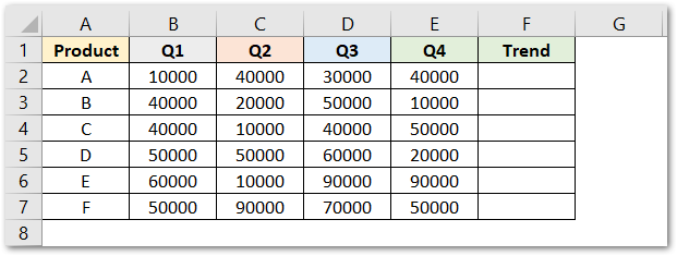
To insert the Line Sparklines in Excel:-

• Select the range of data B2:E7
• Go to Insert tab
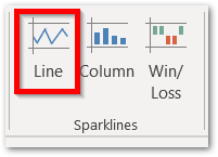
• In the Sparklines group, click on Line sparklines button
• Set the Location range as F2:F7

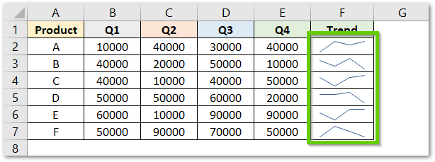
This would insert the Line Sparklines at the required destination as follows.

To format them

• Select the sparklines in cell F2:F7
• Go to Sparkline Tab on the ribbon
• Now choose the desired formatting from the options

Highlighting the Data Points in a Sparkline

The Sparkline is made by plotting the data points in a single cell. In a Line Sparkline, the consecutive data points are joined to form a line sparkline.

Select the Line Sparklines in the range F2:F7 and go to the Sparkline tab on the ribbon.

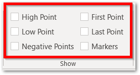
There you will find the options to highlight different data points in the selected sparklines.

• Hight Point – It would mark the highest point of the sparkline.
• Low Point – Marking this checkbox would highlight the lowest point in the sparkline
• Negative Point – Upon marking this checkbox, negative values would be marked in the sparklines
• First Point – This will highlight the first data value on the sparkline
• Last Point – The checkbox would highlight the last point of the sparkline
• Markers – This will highlight all the points in the sparkline

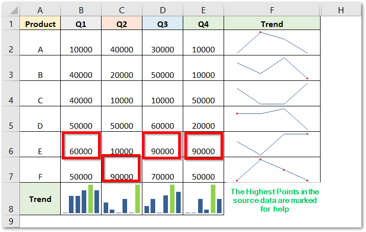
For explaining purposes we have highlighted different parts in each of the sparklines by selecting them one by one.

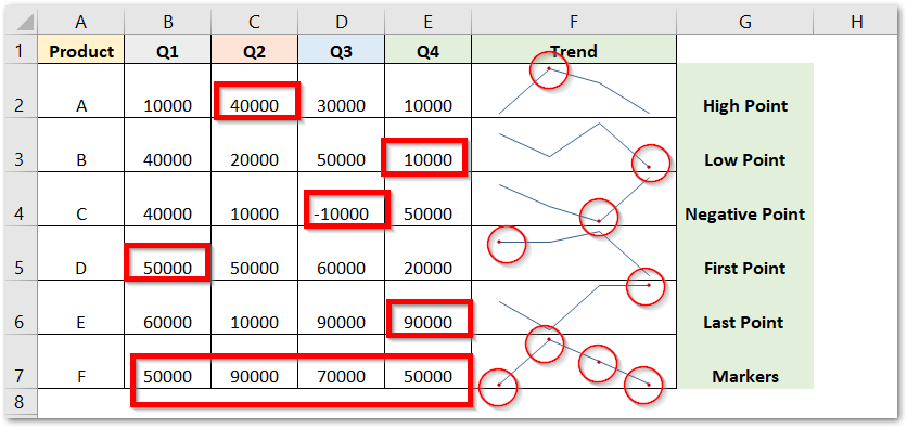
We have marked the highlighted data points in red circles and also marked them in the source data. We have changed the size of sparklines as you can see. This is done by changing the row height and column width of the cell that contains the sparkline.

Formatting the Data Points

As you know in the earlier section we had formatted the sparklines. In a similar way, we can also set the highlighting color for each of the data points in the sparklines. For an example:-

• Select the range of cells B2:E7
• Go to Insert tab on the ribbon
• Choose the Column Sparklines
• The Create Sparkline Dialog box opens.
• Set the location range to B8:E8 and click OK

This would insert the column sparklines below the data. Increase the row height of row 8 to increase the size of sparklines.

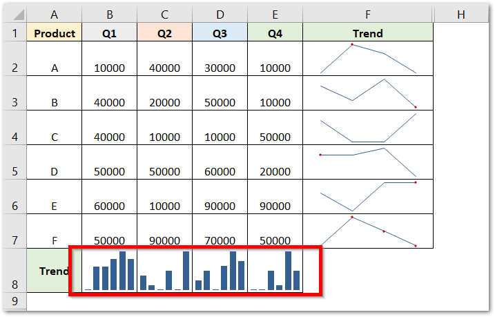
Now select the column sparklines i.e B8:E8 and go to Sparkline Tab on the ribbon.

Mark the check box for High Point in the Show group.

Choose the color for it from here.

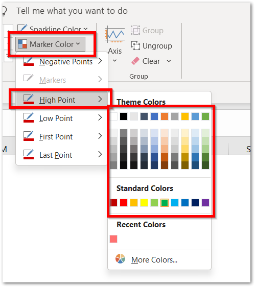
Here you could see that there is an option to set the formatting for all kinds of highlights.

Select the color for the High Points. This is how it would look now.

Fixing the Blanks or Hidden Cells in Source Data

There are times when the source data for our sparklines have blank entries in it. The Line Sparklines in Excel would become noncontiguous as you can see below:-

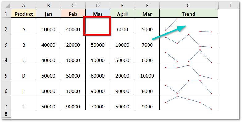
Here you can see that the sale of Product A for March has been left blank. Consequently, its sparkline in cell G2 has become incontiguous.

To change the settings simply:-

• Select the range of cells containing sparklines G2:G7
• Go to Sparkline tab on the ribbon
• Click on the button named Edit Data.
• Choose the option Hidden and Empty Cells

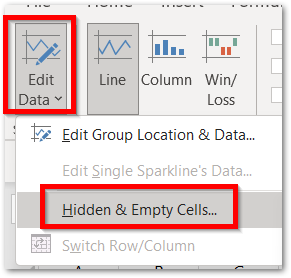
As a result, a dialog box named Hidden and Empty cells Settings would open.

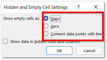
You can either set the blanks to have zero value and its corresponding data point in the sparkline would show zero. Alternatively, we can join the previous and next data points, ignoring the blank entry in the data.

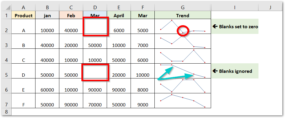
For explaining purposes, we have done both types of settings in each of the sparklines in cells G2 and G5.

Adding an Axis in Sparklines in Excel

When we are using sparklines, there is this minimum value from where the axis begins its scale. These sparklines do not have their scale starting from zero. For instance, check this:-

Here you can see that the minimum value is for January, and it appears as if its value is zero because of the sparkline in cell G2. This is so because the minimum value for the vertical scale of sparkline is set automatically to 95 and the rest of the values are relatively plotted.

We can change this setting, to do so:-

• Select the sparkline in cell G2
• Go to Sparkline tab on the ribbon
• Click on the Axis Button in the Group group.
• Choose the Custom value option for Vertical Axis Minimum value

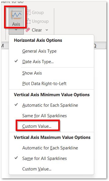
Now fill 0 in the Customs Value. As a result, the vertical axis scale would start from 0.

If you have negative values in the source data of sparklines, then do not set the minimum axis value to zero as the negative values are less than zero and then they wouldn’t show in the sparklines.

Similarly, we can change the Maximum Vertical Axis Value in the Sparklines.

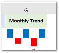
We can even show the horizontal axis for the sparkline, but it would be possible only when the source data has both positive and negative values. For instance, check this:-

To add the axis:-

• Select the sparkline i.e G2
• Go to Sparkline Tab on the ribbon
• Click on the Axis Options button
• Select Show Axis button in the Horizontal Axis Buttons

This is the result.

This brings us to the end of the blog.

Thank you for reading.