In our overview blog on the excel power query feature, we had learned about the basics and the introduction of power query in Excel. We also learned how the power query feature proves to be a useful tool in Excel when you want to get data from other excel sources like PDFs, Text & CSV files, JSON, Websites or web pages, etc. In this blog, we would learn how to use the fill down and fill up feature in excel Power Query.
If you are new to excel power query feature, I strongly recommend you to go through the ExcelUnlocked overview blog on Power Query Feature.
Meaning of Fill Down and Fill Up in Excel (with Examples)
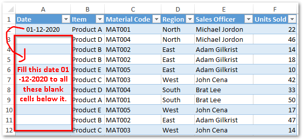
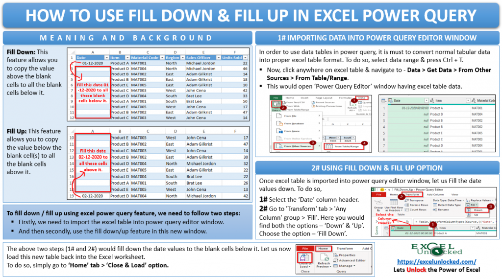
Fill Down: This feature allows you to copy the value above the blank cells to all the blank cells below it.
Fill Up: This feature allows you to copy the value below the blank cell(s) to all the blank cells above it.
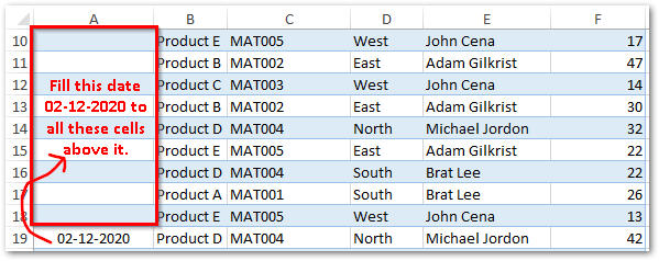
Now, when you know what does fill down and fill up mean, let us begin with this tutorial on how to use this tool in an excel power query.
Fill Down & Fill Up in Excel Power Query [Step by Step Guide]
This involves 2 basic steps:
- Importing data from excel into Power Query Editor window
- Filling the values up or down in the Power Query Editor window
Importing Data from Excel into Power Query Editor Window
In order to import and work with a tabular dataset in power query, it is must that you have an excel understandable table format. The excel power query feature does not understand a normal excel dataset table.
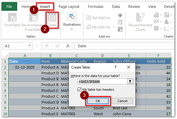
To convert a normal dataset table into an excel understandable table format, select the table range, and then navigate to the ‘Insert’ tab > ‘Table’ group > ‘Table’ option and click OK. Or use the ‘Ctrl + T’ keyboard shortcut.
Now, let us learn how to import this excel table into power query editor window.
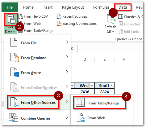
Click anywhere on the table and then follow this path – Data > Get Data > From Other Sources > From Table/Range.
As a result, you would see your excel table in the power query editor window. Also, you would notice that the default name of this window is the Table Name. See the image below.
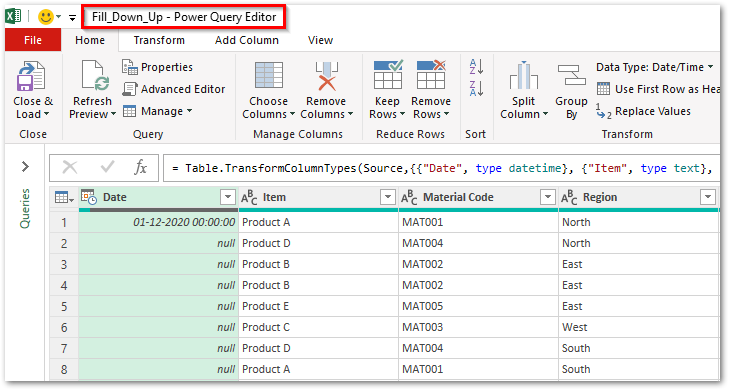
Here, the term ‘Null’ in the Power Query Editor window refers to those cells with no values in it (i.e. the blank cells).
Filling Values Down or Up in Power Query Editor Window
Once the data is imported to Power Query Editor window, follow the below steps:
- Click on the column header ‘Date’ to select the entire column.
- Now, go to the ‘Transform’ tab > ‘Any Column’ group > ‘Fill’. Here you would find both the options – Down and Up. Choose the option ‘Down’ to fill the values down.
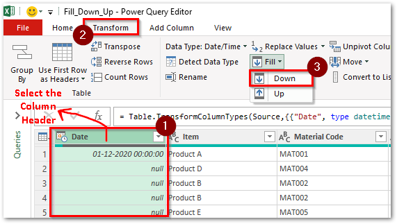
As a result, you would notice it would copy the value above to all the blank cells below in the entire selected column.
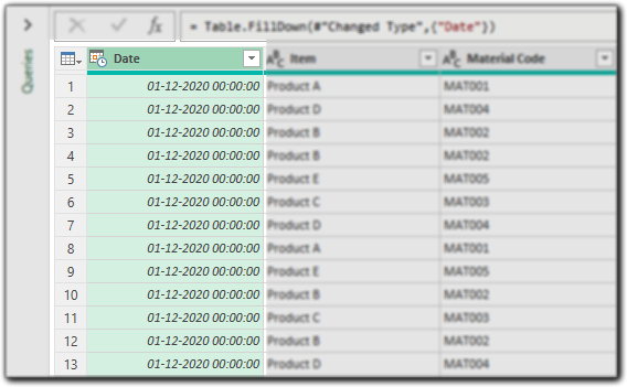
The ‘Date’ column in the transformed table above also shows the time value ’00:00:00′. If you do not need the time, then you can change the column data type from ‘Date/Time’ to ‘Date’. To do so, select the ‘Date’ column, and then go to the Transform tab, click on ‘Data Type: XXXX’ and choose ‘Date’.
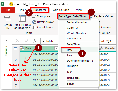
This would instantly, remove the time value ’00:00:00′ from the date column.
This is why I call Excel Power Query feature as a magical life saver tool 😉 So much easy to use with instant results !!
Similarly, you can use the ‘Up’ option under the ‘Fill’ drop-down to copy the value below to all the blank cells above that value.
Importing Table Back from Power Query Editor to Worksheet
Finally, let us import back the new transformed table from power query editor window to excel worksheet.
Go to the ‘Home’ tab > ‘Close’ group > ‘Close & Load’ option (see image below).
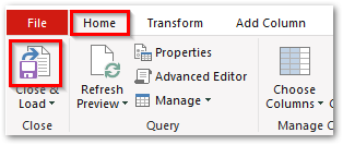
This would instantly load the new table from power query editor window back to excel in a new worksheet.

