In the previous blog, we did the VAR.P Function. In this blog, we would learn the usage of the VAR.S Function in Excel. Both the VAR.P and VAR.S are important statistical functions of excel.
Let’s start learning.
When to Use VAR.S Function in Excel?
The word VAR.S stands for the variance of the sample. The VAR.S formula is used to estimate the variance of data that represents the sample. We use the VAR.P formula if the data represents the entire population.
Variance is a statistical parameter that measures the dispersion of a set of numbers from the average value. Data having a higher value of variance is said to be inconsistent when compared with data of lower variance.
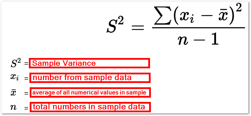
In general, the variance of the sample is calculated using the following formula.
Syntax and Arguments
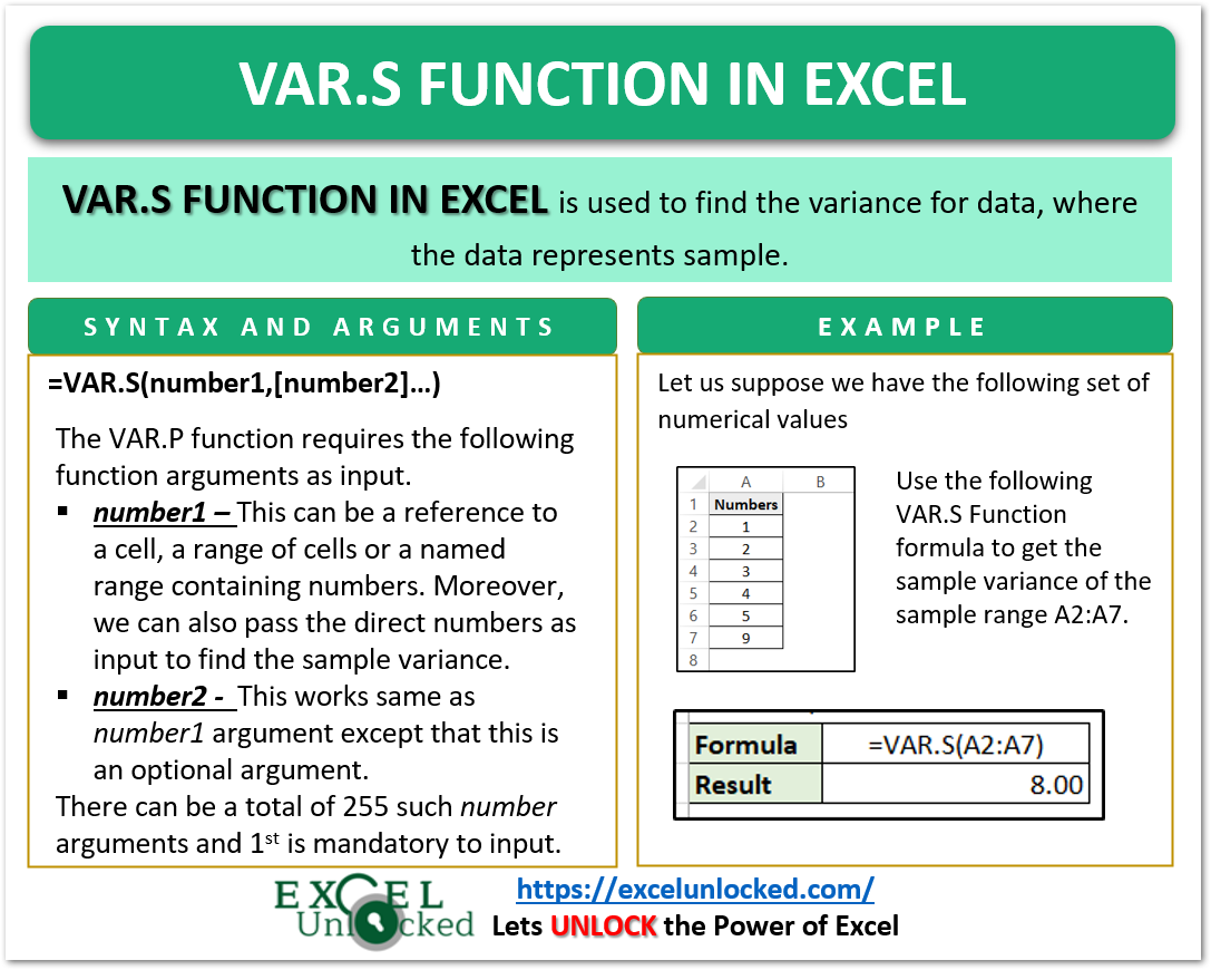
We have to supply the sample data to VAR.S Function in the form of function arguments explained below.
- number1 – This is can be one numerical value or a set of numbers enclosed in brackets. We can pass direct numerical values or use cell references and ranges.
- [number2] – This is an optional argument.
The VAR.S function can be supplied with 255 such total number arguments. Only the first number argument is mandatory to input.
Points to Remember about VAR.S Function
We should always remember the following information about the VAR.S function before implementing the formula.
- The VAR.S function was introduced in Excel 2010 and can be used in later versions also.
- For Excel 2007 or earlier version, use VAR Formula.
- The VAR.S Function ignores the text and logical values referred to by function inputs.
- Arguments can be numbers, arrays or named ranges.
Examples to Implement VAR.S Formula
In this segment of the blog, we will do some examples to learn the VAR.S Function.
Example 1 – Variance using Cell Referencing
In this example, we would start by finding the variance of a sample data set. Let us suppose we have the following numerical data set.
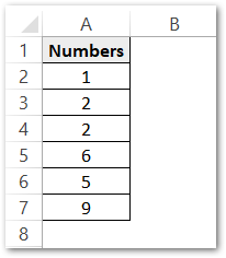
Use the following VAR.S Formula to get the sample variance for this data set.
=VAR.S(A2:A7)
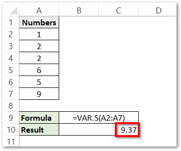
As a result, the formula returns the value of variances as 9.37
Explanation – We have passed the range A2:A7 as the number1 argument of the VAR.S Function input. This array contains the sample set of numbers which is processed by the VAR.S Formula. As a result, we get the value of variance as 9.37
Example 2 – Direct Numerical Array passed into VAR.S Function
In this example, we will use the VAR.S Function when the sample data is not present in excel cells. Let us suppose we have the monthly sales of a business for six months as follows.
{120,142,152,645,124,656}
The sales are written in brackets and separated by comma.
Use the following VAR.S Formula to get the sales variance.
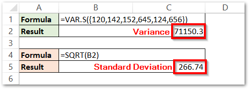
=VAR.S({120,142,152,645,124,656})
As a result, the formula returns sales variance as 72250.3
Explanation – The array of numbers {120,142,152,645,124,656} represents the monthly sales for six months. Here we have passed this array as the number1 argument of VAR.S Formula. As a result, the formula evaluates the sales without referencing any cells. We get the variance as 72250.3
Standard Deviation using Variance
The Square Root of Variance gives the value of standard deviation. When we pass the result of VAR.S function as the input of SQRT Function, we get the value of Standard Devitaion of Sample.
In Example 2, we have calculated the sample variance. Cell B2 contains the result. When we supply this result to SQRT Function, we get standard deviation of the sales {120,142,152,645,124,656}.
=SQRT(B2)
We can evaluate same result by using the STDEV.S Formula to get standard deviation of sample.
This brings us to the end of VAR.S function blog.
Thank you for reading.
