In this blog, we would learn how to merge data in excel from two or more different tables using the Excel Power Query feature.
Difference Between Merge and Append Data in Excel
Merging Data and Appending Data are two different terms and are used for two different purposes. By merging tables in Excel, it means combining two or more excel tables and create one table based on unique records (key field). Whereas, by appending tables in excel, it means to put the table data from two or more excel tables one below the other. It is important to keep in mind that in order to append the tables in excel, the column headers in all the tables should be the same.
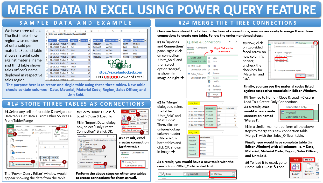
Sample Data for Merging Data in Excel
Suppose we have three tables, as shown in the image below:

The first table shows the region-wise number of units sold per material during the month of December 2020. The second one shows the respective material code against the material number. And the third table shows the sales officer’s name deployed in each of the five regions.
Now, we want to create one single table using these three tables. The new table should contain the following columns – Date, Material, Material Code, Region, Sales Officer, and Unit Sold.
Step by Step Guide To Merge Data in Excel
In order to merge data tables in excel, there are two main activities involved:
- Firstly, to store the three tables as connections
- Merge the connections to create a new table in excel
Let us deep dive into each of these and learn the technique of merging data tables in excel using poower query.
Get Table from Excel File and Store it As Connections
In order to use the get data from a table into the power query, it is must that the dataset table should be a proper excel table. To convert a normal tabular dataset into an excel table, simply select any of the cells within the dataset area, and use keyboard shortcut Ctrl + T. You can find more details about excel table format in this link.
Now, follow the below steps to create connections for tables in power query.
- Select any of the cells in the first table and navigate to the ‘Data’ tab > ‘Get & Transform Data’ group > ‘Get Data’ > ‘From Other Sources’ > ‘From Table/Range’ as shown below:

- As a result, a new window named ‘Power Query Editor’ will pop out on your screen showing the data records of the first table.
- In this window, simply go to Home Tab > Close & Load > Close & Load To as shown below:

- In the dialog box that appears, select the option – ‘Only Create Connections’ radio button and click OK, as shown in the image below:

- As a result, excel would create a connection for the selected table (the first table). You can check this connection in the ‘Queries and Connections’ pane on the right side of the excel work area.

In a similar way, perform all the above steps and create connections for the other two tables (one by one) as well. Finally, you would have three connections listed in the ‘Queries and Connections’ pane, as shown below:

If you are not able to see the ‘Queries and Connections’ pane (image above) in the excel or it is by mistake closed, then you can bring it back by navigating to ‘Data’ Tab > ‘Connections’ group > ‘Queries and Connections’
Merging Power Query Connections to Create One Table
Once we have stored the tables in the form of connections, now we are ready to merge these connections. Follow the undermentioned steps:
- In the ‘Queries and Connections’ pane, right-click on the ‘Units_Sold’ connection and select the option ‘Merge’.

- In the ‘Merge’ dialog box that appears, select the tables ‘Unit_Sold’ and ‘Mat_Code’, as shown below. You can select only two tables at a time for joining.

- The next step is to select the lookup unique columns. In our case, the lookup column is – ‘Material’. Click on the column headers ‘Material’ in both the tables. Finally, click on ‘OK’ as shown below:

- As a result, excels opens up the ‘Power Query Editor’ window. In this window, now you have the new column ‘Mat_Code’ added to the table. Simply, click on the two-side facing arrow on the column header. In the drop-down window that appears, uncheck the checkbox for ‘Material’ and click OK.
- Finally, you can see the material codes listed against respective materials.

- Now, load this table again, as a new connection by navigating to the ‘Home’ tab > ‘Close & Load’ > ‘Close & Load To’ > ‘Only Create Connection’ > OK. As a result, excel creates a new connection for it (as highlighted below).

Now, perform all the above steps to merge this new connection table ‘Merge1’ with the ‘Sales_Officer’ table. As a result of this, you would have a final table ready with you having the new column ‘Sales Officer’, as shown below:

Let us finally, load this table to excel. To do so, Home tab > Close & Load.
That’s it, excel would create a new worksheet with the final data table loaded to it. There are in total of 441 rows of data.

What is So Special About Power Query
The main reason why people choose to use the power query excel feature to import data to excel from other sources is that it is quite easy to use, and no complex coding knowledge is required.
However, apart from its user-friendly interface, the best part of the power query is that the connections stored here at reusable ones.
This means that in an event of any change in the source data table, the power query can incorporate those changes to the table at a click of a mouse.
Let me give you one example to support this. Suppose, I delete a few of the records from the first table – ‘Units_Sold’. Now, I want this change in the source table to get incorporated into the final merged table.
To do so, simply go to the final merged table, right click on any of the cell and select the option ‘Refresh‘.

As a result, excel would perform all the steps one by one and get the latest data.
With this we have completed with this blog on how to merge data in excel from two or more different tables.