Change the Order of Data Series – Stacked Line, Stacked Area, Column Chart

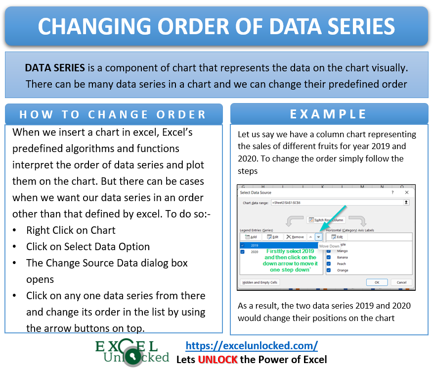
Data Series is the part of the chart representing the source data visually. There are many common types of charts in Microsoft excel including Line Charts, Column Charts, Area Charts, etc. Sometimes, we want our data series to be in a particular order. When we insert a chart, excel’s predefined algorithms define the order of the data series. There can be different ways to change the order of data series of chart in excel. The different chart types can be:-

• Stacked Line Chart of Excel
• Stacked Area Chart of Excel
• Column Chart of Excel

Changing Order of Data Series in Stacked Line Chart of Excel

Let us say we have the following source data:-

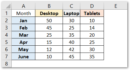
We have inserted a stacked line chart from this source data as follows:-

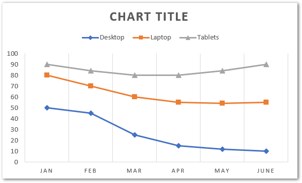
Now as you see that the order of data series plotted is:-

• Desktop
• Laptop
• Tablets

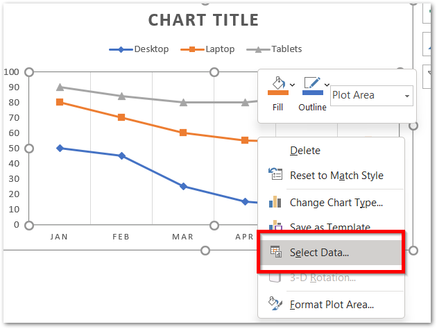
Now to change this order, right-click on this chart and select “Change Data” from the shortcut menu appearing.

Now From the Select Data Source Dialog Box, Select any one data series and hit on up/down arrow to move it and change its order

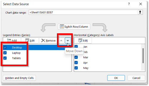
These arrows act as a control to shift and change the order of the data series.

Similarly, we can change the order the of data series in a column chart.

Changing the Order of Data Series in Stacked Area Chart of Excel

In a Stacked Area Chart, the data series form layers like a stack in which the lower data series from the top layer.For instance, look at the 2D Stacked Area Chart and a 3D Stacked Area Chart for the same source data we took in the first part.

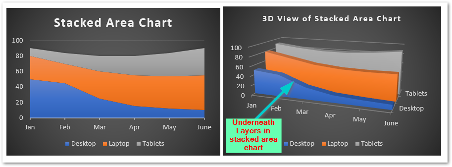
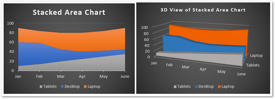
As you can see there is an overlapping of layers. So when we change the order as:-

• Tablets First
• Desktop Second
• Laptops Third

However, to change the order:-

• Right click on the chart
• Choose Select Data
• In the change Source Data Dialog Box, select any one data series
• Use arrows to shift upward/downward to adjust the order of each data series.

This is how the results are:

Changing the Order in Column Chart in Excel

Let us say we have the sales of different fruits for years 2019 and 2020. Therefore, below is a column chart inserted to represent it.

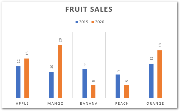
There are two data series in this chart, 2019 and 2020.

As You can see that the adjacent vertical bars represent sales of 2019 and 2020 for each of the axis categories. For instance, the sale of 2019 is represented before the sale of 2020. We can change this order. Right click on this chart and click on the Select Data option.

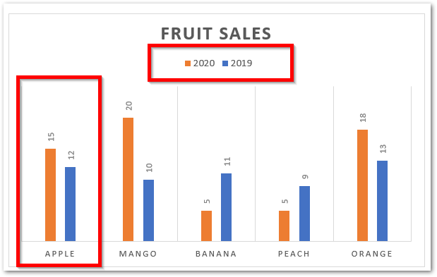
After that select 2019 from the data series and click on the down arrow. This will move the data series 2019 below 2020.

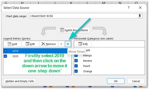
Click OK. As a result, you would see a change of order in your column chart as follows.

This brings us to the end of the blog. 😎

Thank you for reading