Applications of SQRT Function in Excel

In the previous blog, we did the usage of the SQRT Function. In this article, we would cover the practical applications the SQRT Function in Excel.

SQRT Function is a type of Mathematical Function, which is why it can be used in many mathematical formulas and concepts where we have the need to find the square root of a number.

So let’s start learning.

Application 1 – SQRT returning Array of Results ( Excel 365 only )

If you have Excel 365 or Excel 2021, we can use the Excel SQRT Function as the dynamic array formula or simply we can say that the SQRT function can work on an array of cells. An array is a range of cells.

We can use one SQRT function for a range of cells containing numbers. The one formula will spill the results. Consequently, we get the spilled range of results, containing square roots of the input array.

For example, let’s take a range A2:A10.

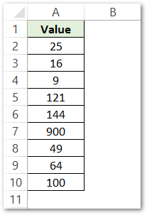
Use the following formula in cell B2 and hit the enter key.

=SQRT(A2:A10)

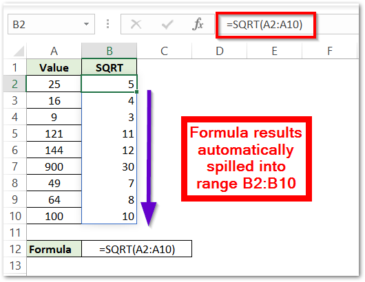
As a result, you can see that the SQRT returns a range of cells B2:B10 containing square roots of the values in the range A2:A10 passed as the SQRT input argument. This is the first application of the SQRT function in Excel.

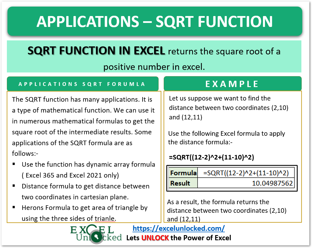
Application 2 – Distance Formula to find Distance Between two Points

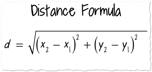
The distance formula gives an equation that calculates the distance between any two points (x1,y1) and (x2,y2) on the cartesian plane.

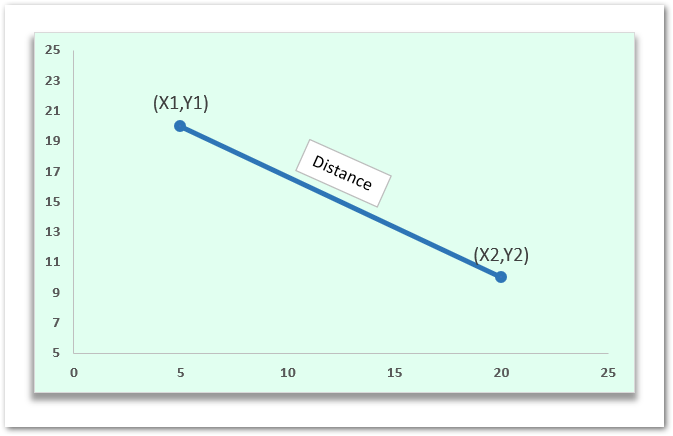
The general equation to calculate this distance is:-

Now let us suppose we have the following pairs of x and y coordinates:-

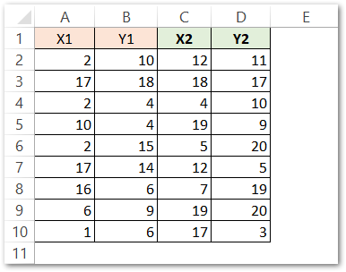
Columns A, B, C, and D contain the values of X1, Y1, X2, and Y2 respectively. Use the following formula in cell E2 to get the distance between (X1, Y1) and (X2, Y2)

=SQRT((C2-A2)^2+(D2-B2)^2)

This carate symbol ( ^ ) gives the power of a number and can be used in place of the POWER function to get the raised to power 2 for the values X2-X1 and Y2-Y1.

Select the range E2:E10. Hit the ctrl D key to copy the formula down the range E2:E10.

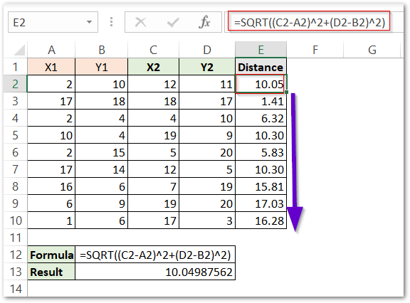
As a result, the formula returns the distance between the respective pair of coordinates in the range A2:D10. And with this, ends one of the important applications of the SQRT function in Excel.

Application 3 – Area of Triangle Using Heron’s Formula

When we have given the length of three sides of a triangle, then we can calculate the area of that triangle by using Heron’s Formula. The general equation of herons formula is:-

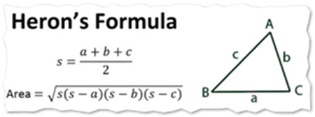
where a,b and c represent the length of the sides of the triangle.

s denotes the semi perimeter.

Now, let us suppose we are given the following triangle dimensions:-

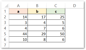
We will start by calculating the value of semi perimeter s by using the following formula in cell D2.

=(A2+B2+C2)/2

Copy this formula down the range D2:D6.

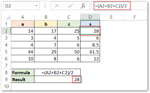
Now we would calculate the area of triangles by using the following formula in cell E2.

=SQRT(D2*(D2-A2)*(D2-B2)*(D2-C2))

Copy the formula down the range E2:E6.

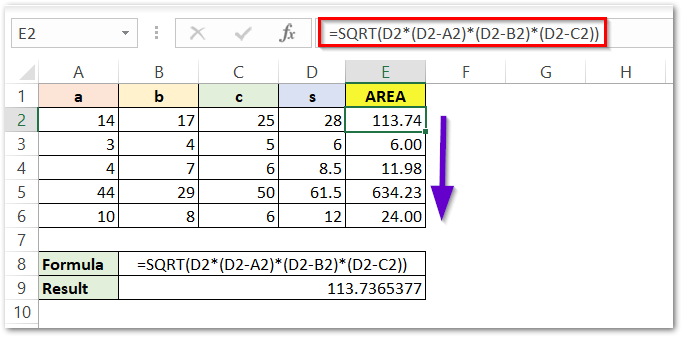
As a result, the formula returns the area of five different triangles in the range E2:E6. This was the third application of the SQRT function in Excel. There can be numerous such applications of the SQRT formula where we want to find the square root of a number.

This brings us to the end of the blog.

Thank you for reading. 😇