The SIN Function in Excel is an essential type of Mathematical Function The function is easiest to learn and implement. So let us begin learning the process.
When to Use SIN Function in Excel?
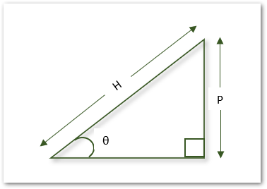
The SIN Function calculates the value of a Trigonometric function known as Sin θ. In a right angle triangle, Sin θ refers to the ratio of the side opposite to angle θ and the hypotenuse
Sin θ value is given by:-
Sin θ = P/H
Where P and H are the lengths of the Perpendicular and Hypotenuse respectively.
Here θ represents the angle for which we want to get the value of the Sin Function. This angle must be in radians for the SIN Function to work correctly.
Syntax and Arguments
=SIN(number)
The SIN Function requires only one function input to implement which we have explained as follows:-
- number – This is the actual angle represented above as θ for which we want to get the value of the SIN function. It must be an angle measured in radians.
Important Points about SIN Function
Here are some important notes regarding the SIN Function in Excel.
- The number argument must be an angle in radians and not in degrees. We can convert the degrees into radians by two methods:-
- Use the RADIANS Function =RADIANS(270)
- Multiply the degree value with PI()/180
- The result of the SIN function always lies in the interval [-1,1]
- The SIN Function came into existence in excel 2007 and cannot be used in earlier versions.

Examples to Find Sin θ value in Excel
In this section of the blog, we would now implement the SIN Function.
Example 1 – Basic Example for SIN Function
Let us suppose we have the following values of Angles in degrees for which we want to get the value of the Sin Function.
Also Read: COS Function in Excel – Usage with Examples
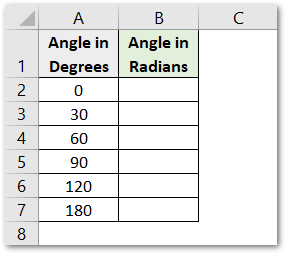
Use the following RADIANS function formula in range B2:B7 to first convert the angle from Degree to Radian
=RADIANS(A2)
Copy the formula down the range B2:B7.
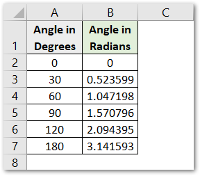
Since we have now got the angle converted into radians in range B2:B7, we can now implement the SIN Function in cell C2.
=SIN(B2)
Copy the formula for the rest of the angles.

As a result, we have got the value of the SIN Function in excel.
Explanation – We have first converted the degree into radians for the angle. This can be done with RADIANS Function or with the help of the PI() Function. Next, we have supplied the result of the RADIANS Function as the number argument of the SIN Function which in return gives us the required results.
We can also use the following formula if we do not need the angle in radians in column B.
=SIN(RADIANS(A2))
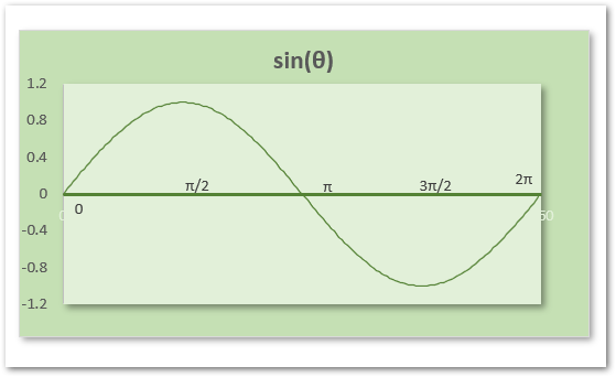
The graph of the SIN Function is as follows.
Example 2 – Finding the Height of the Building using the SIN Function
Let us suppose we have the following imagination of a building and sun.
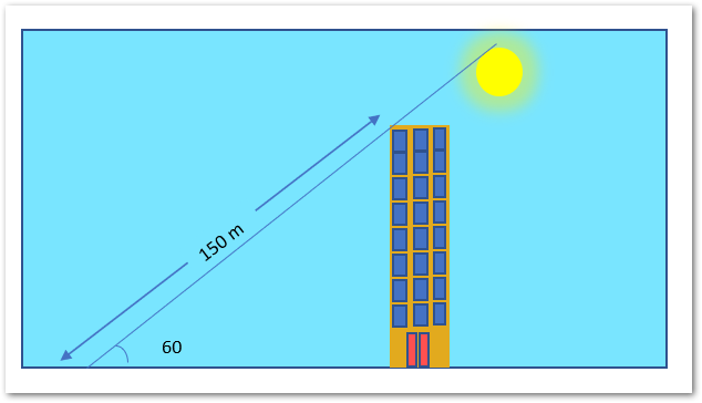
The length of the shadow of the building is 150 m and the angle of the sun’s rays is 60 degrees.
We are willing to find the height of the building. Use the following formula to get the value of SIN 60.
=SIN(RADIANS(60))
As a result, we would get 0.87

As Sin is the ratio of Perpendicular to Hypotenuse. Here Perpendicular is Building and Hypotenuse is the sun rays.
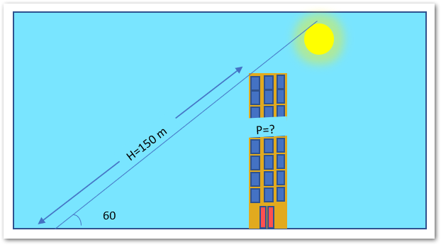
P=H*SIN(RADIANS(60))
Now we can use the following formula for getting the Height of the building.
=150*SIM(RADIANS(60))
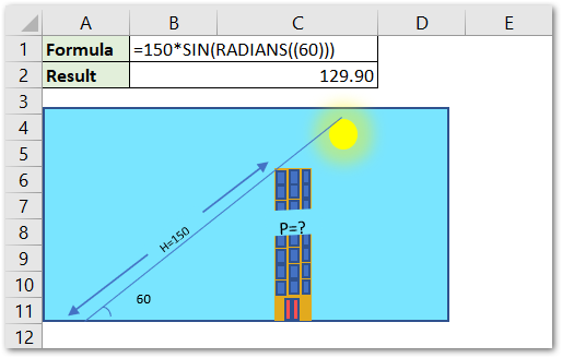
As a result, we got the height of the building to be 120.9 meters.
This brings us to the end of the SIN Function blog.
Thank you for reading.
