In the previous blog, we used the MMULT Function to multiply two matrices. In this blog, we will learn another important function that works on a matrix. Matrix is simply a range of cells in Excel. MINVERSE Function in Excel is a type of Mathematical Function.
So let’s get started.
When to use MINVERSE Function in Excel?
The word MINVERSE means Matrix INVERSE. The MINVERSE function finds the inverse of a square matrix. The number of rows and columns is equal in a square matrix. The resultant inverse matrix is of the same order as the actual matrix.
It is possible where finding the matrix inverse is not possible. This happens when the determinant of the input matrix is equal to zero. So in this case, the MINVERSE function returns a #NUM! error.
Syntax and Arguments
=MINVERSE(array)
The MINVERSE function needs only one input as mentioned below.
- array – This can be a range of cells containing numbers, a named range or hardcoded numbers. We can directly pass the numerical values of the matrix in curly brackets {} with commas in between the numerical values.
This array must be a square matrix. Alternatively, we can say that the order of the matrix must be m*m. For example, a 2*2 matrix would contain 2 columns, 2 rows and 4 elements.
A 3*3 matrix would contain 3 columns, 3 rows and 9 elements.

Important Points about MINVERSE Formula
Before you actually start using the MINVERSE formula, the following information about this function must be known to you.
- The MINVERSE Function works only on a square matrix. Otherwise, the MINVERSE Function returns a #VALUE! error.
- MINVERSE formula needs to be handled differently if you have excel 2019 or an earlier version. After typing the formula, press the ctrl shift enter key. This will spill the matrix inverse result into a number of cells as it is an array formula. You need to explicitly press the ctrl shift enter key to get the matrix inverse result.
- You will get a #NUM! error for a matrix whose determinant is zero.
- If the array input contains any non-numerical value or a blank cell then the formula returns a #VALUE! error.
Examples to Learn MINVERSE Function
In this section of the blog, we would do some examples to implement the formula.
Example 1 – Finding Inverse of 2 X 2 Matrix
Let us suppose we have the following range of cells.

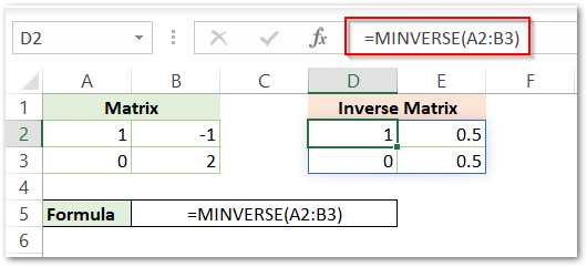
The matrix is the range A2:B3 and is of order 2 X 2.
We want to find its inverse matrix. Type the following formula in cell D2.
=MINVERSE(A2:B3)
After typing the formula, press the ctrl shift enter key to get the result of the matrix inverse,

As a result, you can see that the formula has successfully returned matrix inverse in the range D2:E3.
Explanation – We have supplied the range A2:B3 as the array input of the MINVERSE Formula. After typing the formula, once we hit the ctrl shift enter key, the formula returns the resultant inverse matrix in the spilled range D2:E3.
Example 2 – Inverse of a 3 X 3 Matrix
Let us suppose we have the following range of cells.

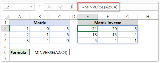
Type the following formula in cell E2.
=MINVERSE(A2:C4)
Hit the ctrl shift enter key.

As a result, the function returns the inverse matrix of order 3 x 3 in range E2:G4.
This brings us to the end of the blog.
Thank you for reading.
