ISODD Function in Excel – Conditional Formatting

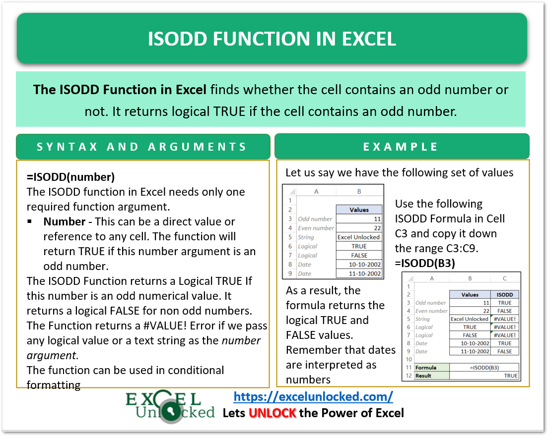
The ISODD function in excel is one of the Information functions in Excel. The information function returns information regarding the cell content we pass as the Information Function Argument.

So let’s start learning about the ISODD formula.

When to use ISODD Function in Excel?

As the name suggests to you, the ISODD function returns a logical TRUE or FALSE based on the condition of whether the supplied cell content contains an odd number or not.

Not to be mentioned, numbers not divisible by 2 are odd numbers i.e. 1,3,5,7 and so on.

• The ISODD function returns a TRUE when we pass an odd number i.e =ISODD(1) gives TRUE
• The Function returns a FALSE when we supply an even number i.e =ISODD(2) gives FALSE

The ISODD function works fine with the numbers formatted as text.

ISODD function returns #VALUE! error if we pass text strings or logical values as function argument number

Syntax and Arguments

=ISODD(number)

The ISODD Function requires only one function argument is:

• number – This can be a direct value or reference to any cell. The function will return TRUE if this number argument is an odd number.

This function has some irreplaceable usages we have covered in the examples section.

Examples to Learn ISODD Formula

In this section, we have performed some practical experimentation with the ISODD Function:-

Example 1 – Simplest Example for ISODD formula

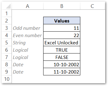
Let us suppose we have the following set of values in the range B3:B9.

Use the following formula in cell C3.

=ISODD(B3)

Now select the range C3:C9 and press the Ctrl D key to copy the formula down the range C3:C9.

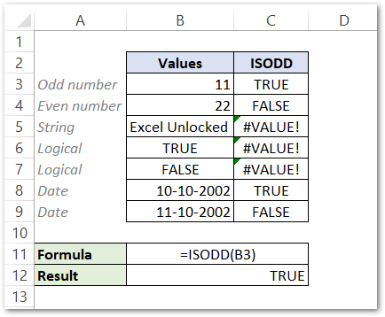
As a result, you can see that the function returns TRUE and FALSE for 11 and 22 respectively. B5:B7 contains text strings and logical values which is why the formula returned #VALUE! error.

The Dates ( B8, B9 cell ) in Excel have their numerical values in the backend. For Example 1 Jan 1900 is read as 1, 2 Jan 1900 is read as 2, and so on. The values for 10-10-2002 and 11-10-2002 are 37539 (odd – TRUE ) and 37540 ( Not odd – FLASE ) respectively. The ISODD Function works on the numerical values of these dates.

Example 2 – Highlighting the cell containing Odd numbers

Let us suppose we have the following set of values:-

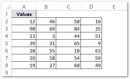
We want to highlight the cells that contain odd numbers. We are going to use Conditional Formatting for this purpose.

To apply conditional formatting on the range A2:D8 simply:-

• Select the range A2:D8
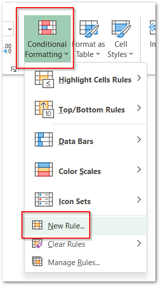
• Go to the Home tab and click on the Conditional Formatting button. Choose New Rule from the list.

• This opens the New Formatting Rule Dialog box. Choose the option Use a Formula to determine which cells to format.

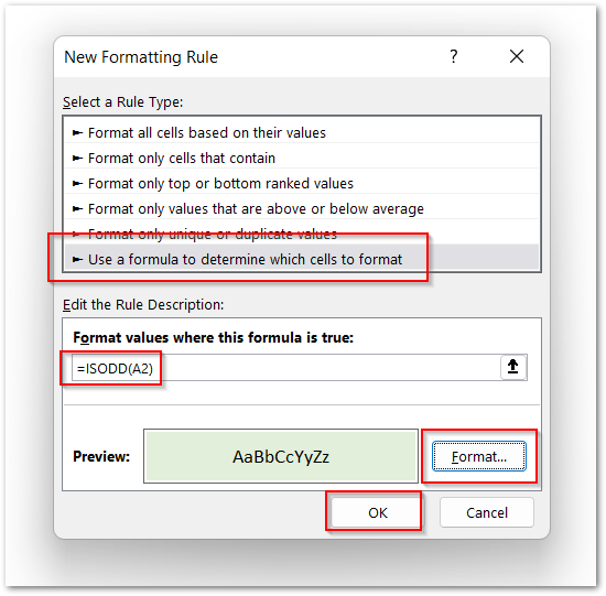
• Enter the ISODD formula in the New rule. Set the Format of the cells if ISODD returns a logical TRUE as fill to green and click Ok. ( Step 4 marked )

=ISODD(A2)

As a result:-

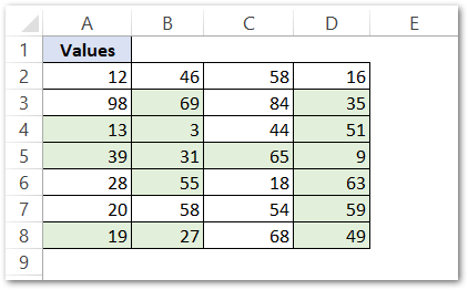
All the odd values in the range A2:D8 have been highlighted with a green solid fill.

Example 3 – Filling The Alternate Rows using the ISODD and ROW Function

Let us suppose we want to have the following cell formatting of the rows:-

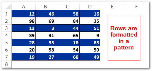
Here the first row 1 is formatted while the next row 2 is unformatted. In this way, the rows are formatted in a pattern. We can do this in a fraction of seconds to the unformatted range:-

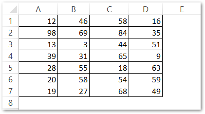
• Select the Range of cells A1:D7. Repeat all the steps as mentioned in Example 2 Except:-
• Use the following formula in the New Formatting Rule box ( Step 4 )

=ISODD(ROW(A1))

• Set the Format as Blue Solid fill, White Font, and Bold

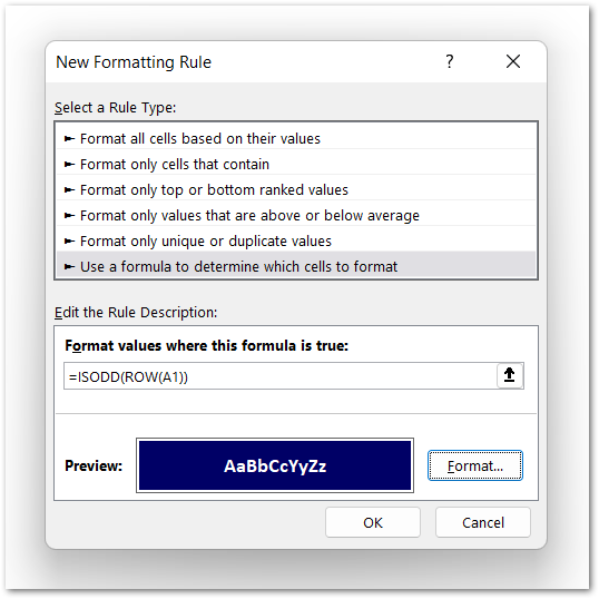
As a result, the formula highlights the odd rows.

We can also use the formula =ISEVEN(ROW(A1)) to highlight even rows

This brings us to the end of the blog.

Thank you for reading.