Excel Gridlines

Do you know what is an Excel Gridline? In this blog, we would understand the definition of Gridlines in Excel and other related settings and functions. As you would proceed with this blog, you would unlock also learn various other interesting things like printing the gridlines, changing the color of the gridlines and many more such things.

What is an Excel Gridline?

Excel Gridlines are the faint grey colored lines that are available in a worksheet.

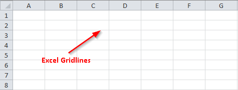
Moreover, the intersection of the Excel gridlines in the excel makes a cell.

Delete the Gridlines from Single Worksheet?

By default, Excel always shows the gridlines when you open any new workbook. To remove the gridlines from a worksheet, follow the steps as described below:

Step 1: Go to the worksheet in which you want to remove the gridlines.

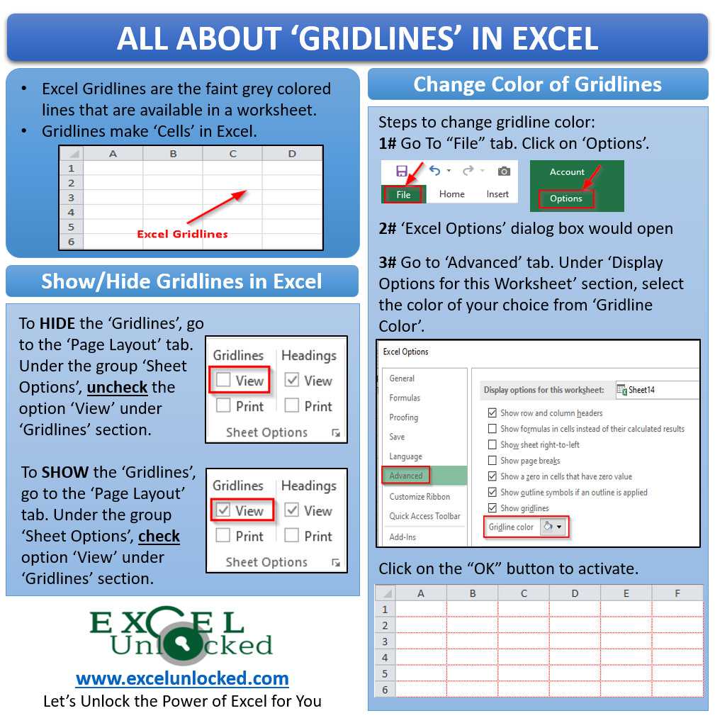
Step 2: In the Excel ribbon, click on the tab “Page Layout”. Under the group “Sheet Options”, uncheck the “View” checkbox in the “Gridlines” section of this group.

As a result, you can see that gridlines disappear from the Excel worksheet.

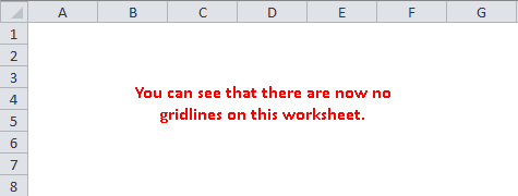
Now to make the gridlines visible, again select the ‘View’ checkbox. And your Excel gridlines would be visible.

There is another way/path to show or hide a gridline in Excel. Go to the ‘View’ tab in the Excel Ribbon Bar. Under the group ‘Show’, you would see a checkbox named ‘Gridlines’ (which is checked by default). Uncheck this checkbox to hide the Gridlines.

Using Keyboard Shortcut to Hide/Remove Excel Gridlines

Rather than using the above methods, you can even use the keyboard shortcut to hide or remove the gridlines from an Excel Worksheet.

Use keyboard shortcuts Alt + WVG. 

Delete Excel Gridlines from Multiple Worksheets Quickly?

By default, Excel would only remove the gridlines from the active method (using the above method).

In order to remove the gridlines from the multiple worksheets at one click, you need to first group the sheets.

In order to group multiple worksheets, click the Ctrl key on your keyboard and then click on the worksheet tabs to the group.

The grouped worksheets would look like this. I have group Sheet 1, Sheet 2, Sheet 3 and Sheet 4, as can  be seen from the screenshot below:

Now, go to the “Page Layout” tab in the Ribbon. Under the group “Sheet Options”, uncheck the “View” checkbox in the “Gridlines” section.

As a result, you can see that there are no gridlines in all the worksheets.

Printing Gridlines

By default, Excel does not print the gridlines. However, to print the excel gridlines, you need to make the following settings in Excel.

In the Excel ribbon, click on the option ‘Page Layout’. Under the group “Sheet Options”, check the “Print” checkbox in the “Gridlines” section.

Changing Gridline Colors

Whenever you would open any new excel workbook, you would notice that the color of the gridlines in excel is ‘Grey’. This is the default color.

To change this default color, go to the worksheet for which you want to change the gridline color. 

Now follow the below steps:

Go to the “File” tab. Click on the”Options” button.

The “Excel Options” dialog box would appear.

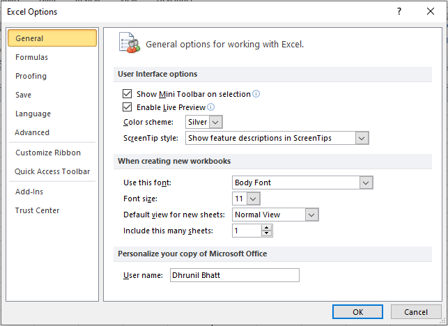
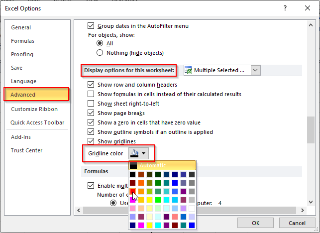
Select the option “Advanced” on the left side of this dialog box and then scroll down to reach the section “Display option for this worksheet”.

In the “Display option for this worksheet” option, select the color of your choice from the “Gridlines Color” option and click on the “OK” button:

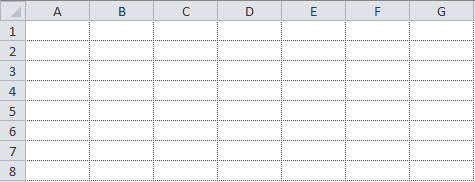
You would notice that the color of the gridlines in the worksheet gets changed to the selected color as shown in the screenshot below:

This brings us to the end of this blog.