MOD Function in Excel – Find Remainder after Division

Excel MOD function is a mathematical formula in excel which is used for finding remainder from division in excel.

In this tutorial, we would learn how to use the excel MOD function along with its syntax, arguments, simple examples, and some real-life practical examples.

This tutorial will help you to understand how the MOD formula works in excel.

So, let us begin 😎

When to Use MOD Function in Excel

The MOD excel formula got its name by its function in mathematics – ‘Modulo operation’ or ‘Modulus’.

It is a mathematical operation that is useful to get the remainder by dividing one number (i.e. dividend) by another number (i.e. divisor). It returns a number as a result of the division in excel.

This formula is very useful to answer the following common excel question

• How to do division of numbers in excel?
• How to divide numbers in excel?

Syntax and Arguments

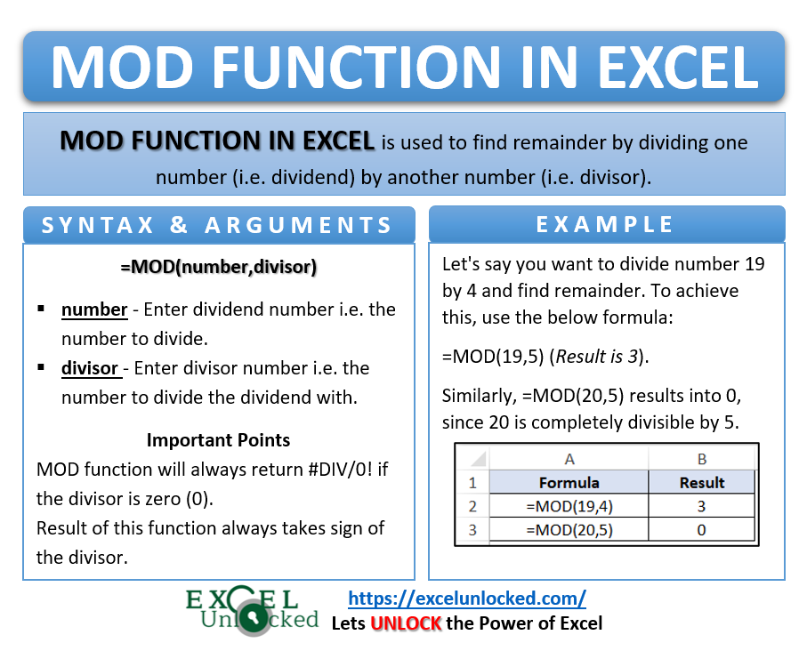
=MOD(number, divisor)

This function has following two arguments:

• number – In this argument, enter the dividend number i.e. the number to divide.

• divisor – In this argument, enter the divisor number i.e. the number to divide the dividend with.

Simple Example – Using MOD Formula in Excel

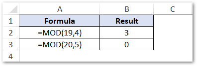
Let’s say you want to divide the number 19 by 4 and find remainder.

To achieve this, simply use the below formula:

=MOD(19,5)

As a result, excel returns the result ‘3’ which is nothing but the remainder resulting by dividing 19 with 4.

Similarly, =MOD(20,5) results into 0, since 20 is completely divisible by 5.

Do Not Miss These Points

• The input arguments of the MOD excel formula can be entered manually (as learned above), or given as a reference to another cell or formula.

• MOD function will always return #DIV/0! if the divisor is zero (0). The reason for #DIV/0! error in excel is very simple. Mathematically, you can not divide any number by zero, and hence this error occurs in the MOD function as well.

• The MOD function resultant remainder always takes up the sign of the divisor. For example – Division of a number with a negative number using MOD function will result in a negative number.

How is MOD Function Practically Used in Excel?

Now, when you have a clear understanding about what is the purpose MOD excel formula and how it works, let us see some practical aspects of the excel MOD function.

Ex. 1 # Highlight Every Nth Row in Excel

The MOD function is a heart for highlighting Nth row in excel with a color.

Using a combo of MOD function and conditional formatting excel feature helps in highlighting every alternate (2nd), third (3rd), fourth (4th) row, and so on.

I have prepared a detailed tutorial/blog on how to highlight the alternate rows in excel to learn it in more detail.

Ex. 2 # Highlight Every Odd Row or Even Row in Excel

Again, by the using the combination of MOD formula and conditional formula, you can color every odd or even row in excel.

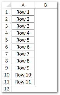
Let’s take the below example dataset.

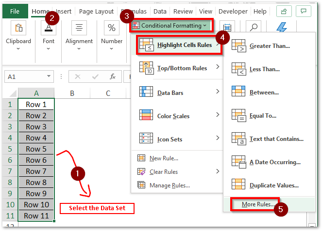
Firstly, select the dataset and then navigate to Home tab > Conditional Formatting > Highlight Cells Rules > More Rules. See image below:

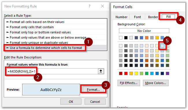
In the ‘New Formatting Rule’ dialog box, select the option – ‘Use a formula to determine which cells to format.

In the formula input box, enter the the following and select the fill color of your choice.

=MOD(ROW(),2)=1

All the above steps are shown in the image below.

After performing above steps, click OK.

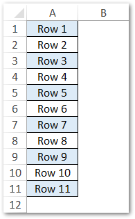
As a result, excel would fill the odd cells with the selected color as shown in the below image.

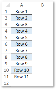
Similarly, to highlight every even cell in excel all the steps learned above remains the same, with an only change in the formula:

=MOD(ROW(),2)=0

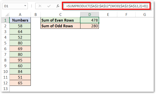
Ex. 3 # Sum or Add Only Odd Numbers or Even Numbers in Excel

The combined usage of the SUMPRODUCT excel function along with the MOD formula helps in adding every odd/even numbers in excel.

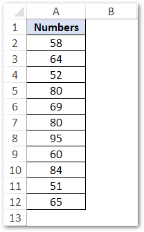
To add or sum only even numbers, use the below formula:

=SUMPRODUCT($A$2:$A$12*(MOD($A$2:$A$12,2)=0))

Similarly, to add or sum only odd numbers, use the below formula:

=SUMPRODUCT($A$2:$A$12*(MOD($A$2:$A$12,2)=1))

Finally, we have completed this blog on MOD function in excel. Thank You. 🙂