In the previous blog, we did the usage of the GCD formula to calculate the Greatest Common Divisor. LCM Function in Excel is also a type of Mathematical Function. The function is the easiest to use. Let’s start learning.
When to use LCM Function in Excel
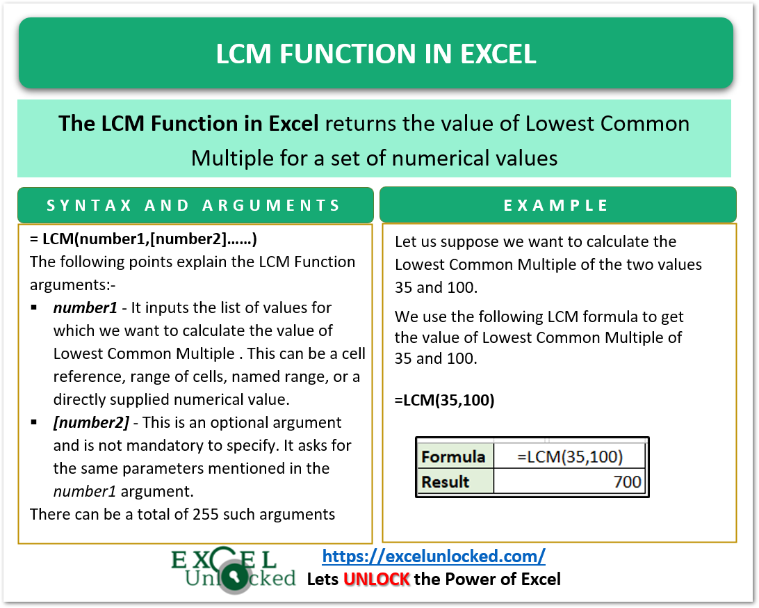
The function name must have suggested to you, LCM Function calculates the Lowest Common Multiple for the set of numbers. LCM is the smallest possible multiple of all the numbers in the set.
Here, let us suppose we have the first five multiples of 20 and 25.
| Multiples of 20 | Multiples of 25 |
| 20 | 25 |
| 40 | 50 |
| 60 | 75 |
| 80 | 100 |
| 100 | 125 |
Here you can see that the minimum value of a common multiple of 20 and 25 is 100. i.e 20×5=100 and 25×4=100.
Although we can have other common multiples of 20 and 25 like 200 i.e 20×10=200 and 25×8=200, but we will consider the smallest value of the common multiple of the two numbers.
Also Read: GCD Function in Excel – Usage with Examples
Therefore, the LCM of 20 and 25 is 100.
Syntax and Arguments
=LCM(number1,[number2]…….)
Below, we have explained the required function inputs for the LCM Function in Excel.
- number1 – This represents the first value of the set of numerical values. It can be a direct value, cell reference, a range of cells containing a set of numerical values, or a named range.
- [number2] – This is an optional argument. It works the same as a number1.
There can be 255 such number arguments. Out of all these arguments, only the first argument number1 is mandatory to specify for normal function implementation.
Important Points to Remember About LCM Formula
Before we actually implement the LCM Function, it is mandatory to know the following notes about eh LCM Function.
- The function operates only on integer values. The digits after the decimal would be truncated by the function while calculating the LCM.
- A #NUM! error is returned by the function if we pass a non-numerical value as the LCM’s input.
- When you pass a text string to the LCM Function, it returns a #VALUE! error.
- LCM function considers blank cells as zero.

Examples to Learn the LCM Function
In this section of the blog, we would perform practical experimentation with the LCM formula.
Example 1 – -Basic Example for LCM Function
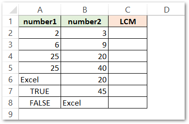
Let us suppose we are having the following pairs of numbers in columns A and B.

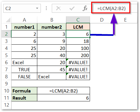
Use the following formula in cell C2, to get the LCM of numbers in cells A2 and B2:-
=LCM(A2,B2)
Alternatively, you can also use:-
=LCM(A2:B2) //A2 and B2 cell passed as range
Once you have entered the formula in cell C2, select the range C2:C8 and press the ctrl D key to copy the formula for all other pairs of numbers.

As a result, the formula has returned the LCM of 2 and 3 as 6.
Explanation – We have passed the range A2:B2 as the number1 argument in the formula =LCM(A2:B2). The function calculates the Lowest Common Multiple of the two numbers in the range A2:B2 and returned the result. The cells C6, C7, and C8 contain the #VALUE! error because we passed nonnumerical values as the function argument ( A6=”Excel”, A7=TRUE, A8=FALSE, and B8=”Excel”).
Example 2 – Finding LCM of More than Two Numbers
In this section, we would try to find out the LCM of more than two numbers in one go.
Let us suppose we want to find the LCM of 10, 12, 14, and 28. We can directly pass the inputs as numerical values to the LCM function.
=LCM(10,12,14,28)

As a result, the LCM formula returns the LCM of the numbers as 420.
This brings us to the end of the blog.
Thank you for reading.
