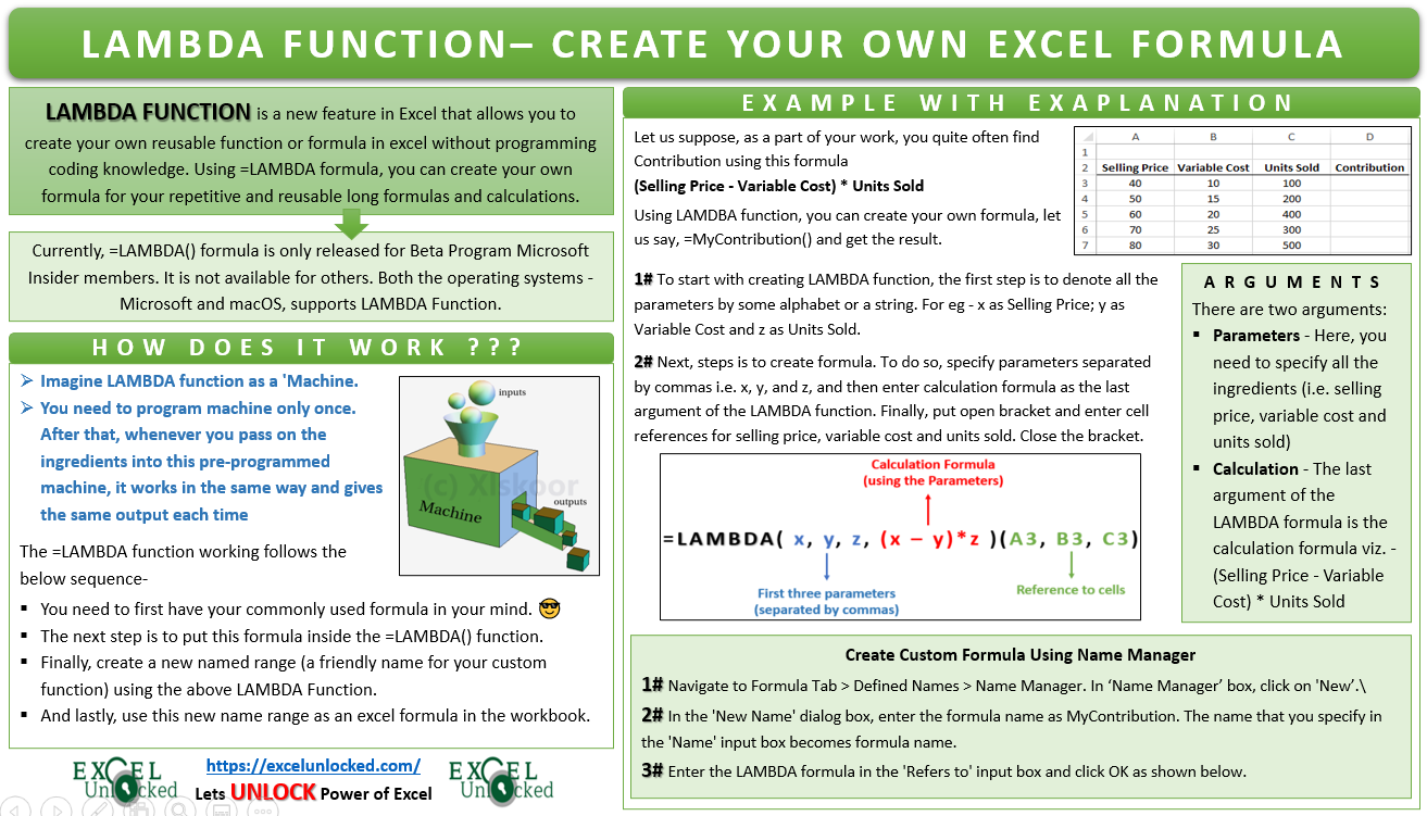
LAMBDA Function – Create Custom Formulas in Excel

LAMBDA function is a new feature in Excel that allows you to create your own reusable function or formula in excel without programming coding knowledge. This new function has the ability to use Excel’s own formula language to create our own custom formula. There is no need of having any programming or VBA knowledge to use this function. Even a non-programmer, like me 😉 can use it very easily.

Using =LAMBDA formula, you can create your own formula for your repetitive and reusable long formulas and calculations.

In this blog, we would learn how to use the new LAMBDA function in Excel along with some examples.

Compatibility of LAMBDA Function in Excel Versions

• Currently, the =LAMBDA() formula is only released for Beta Program Microsoft Insider members. It is not available for others.
• It is available for both the operating systems – Microsoft and macOS.

How does LAMBDA Function Work?

Imagine the LAMBDA function as a ‘Machine’.

You need to program the machine only once. After that, whenever you pass on a set of ingredients into this pre-programmed machine, it works in the same way and gives the same output each time.

The =LAMBDA function works in a similar way.

The =LAMBDA function working follows the below sequence-

• You need to first have your commonly used formula in your mind. 😎
• The next step is to put this formula inside the =LAMBDA() function.
• Finally, create a new named range (a friendly name for your custom function) using the above LAMBDA Function.
• And lastly, use this new name range as an excel formula.

Let us unlock each of the above steps one by one with example on LAMBDA function.

Simple Example to Understand Excel LAMBDA Function

Let us suppose, as a part of your job you have to repetitively calculate the total contribution margin using the below formula:

(Selling Price – Variable Cost) * Units Sold

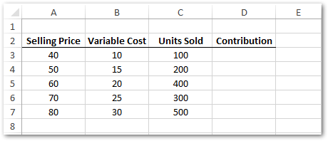
Using the LAMBDA function, you can create your own machine, let us say, =MyContribution() and pass the required three ingredients in it which are selling price, variable cost, and units sold to get the calculated result. This we will see in the latter part of this blog.

Let us first begin with understanding the LAMBDA Function syntax and arguments.

Formula Arguments and Syntax

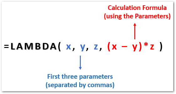
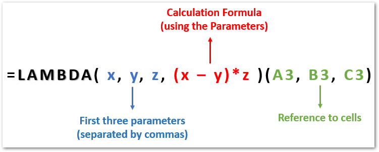
For easy understanding, I would like to divide the entire LAMBDA Function into two sections:

1. Parameters – Here, you need to specify all the ingredients. In our case, there are three ingredients – selling price, variable cost, and units sold. Each of these parameters should be separated by a comma.
2. Calculation – The last argument of the LAMBDA formula is the calculation formula which is (Selling Price – Variable Cost) * Units Sold.

How to Use and Create LAMBDA Formula?

To start with creating LAMBDA function, the first step is to denote all the parameters by some alphabet or a string.

For simplicity purpose, I am using alphabets – x, y and z, where;

• ‘x’ denotes Selling Price;
• ‘y’ denotes Variable Cost; and
• ‘z’ denotes Units Sold

You may use any other strings of your choice, like ‘SP’ for selling price, ‘VC’ for variable cost, and ‘US’ for Units sold.

Let us now built our LAMBDA function in Excel, as shown below-

• Specify the ingredients (i.e. parameters) separated by commas i.e. x, y, and z.
• And finally, enter the calculation formula as the last argument of the LAMBDA function.

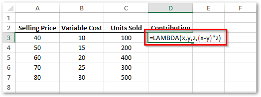
As soon as you prese Enter, you would notice that excel gives an error 🙁 But why?

The reason for the LAMBDA function giving the excel formula error is that we have yet not specified the values for x, y, and z.

To do so, enter the cell references for selling price, variable cost and units sold, within parenthesis, each of which is separated by comma, as shown below:

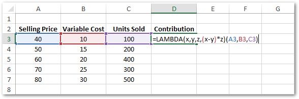
Now when you press Enter, you would get the correct results, without any excel error. 😉

Copy this formula to other cells below it to get contribution margin for each of the rows.

Let us now learn how to create our own formula with the name =MyContribution() and easily calculate Contribution.

Create Custom Formula Using Name Manager

Follow the below steps for creating own custom formula using named range:

• Navigate to the ‘Formulas’ tab and select the option – ‘Name Manager’ under the ‘Defined Names’ group, as shown below:

• As a result, in the ‘Name Manager’ dialog box, click on ‘New’ option as highlighted below.

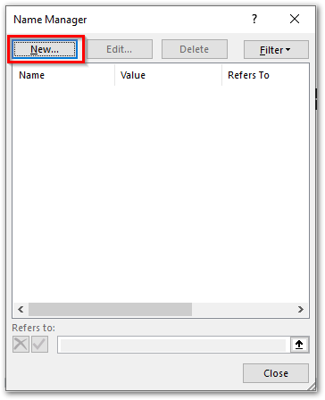
• In the ‘New Name’ dialog box, enter the formula name as MyContribution. The name that you specify in the ‘Name’ input box becomes formula name.

• Enter the LAMBDA formula in the ‘Refers to’ input box and click OK as shown below.

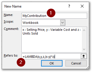
That’s it !! Finally, the custom function with the name MyContribution is ready for use.

Testing the New Custom Formula in Excel

Press ‘=’ on your keyboard and start typing the newly created name – ‘MyContribution‘. As a result, you would notice that excel would suggest you with the custom formula.

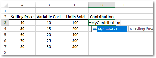
Finally, select the cell references of the three parameters separated by commas, like this,

=MyContribution(A3,B3,C3)

As soon as you press enter, you would get the result as 3000.

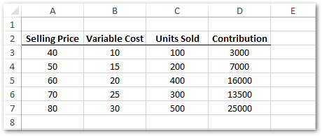
Thus to conclude, the LAMBDA function allows you to create a small formula for repetitively used long formulas.