In our previous blogs, we had seen how to use the RAND and RANDBETWEEN function in excel to generate random numbers in a cell or range of cells. In this tutorial, we would learn another excel formula to generate random numbers viz. excel RANDARRAY function.
The excel RANDARRAY formula is an advanced version of the RAND and RANDBETWEEN excel functions. This function is currently only available for Microsoft excel Office 365 users. Therefore, RANDARRAY is not available in prior versions of Excel – Excel 2010, Excel 2016, and Excel 2019.
In this tutorial, we would learn how to use the RANDARRAY excel function along with examples.
When to Use RANDARRAY Excel Function
The RANDARRAY formula in excel is a math/trig function that is useful for generating random numbers in a specific cell range or an array.
Depending on the input argument this function either returns an array of random whole numbers or integer values.
Syntax and Arguments
=RANDARRAY([rows],[columns],[min],[max],[integer])
All the five input arguments of the excel RANDARRAY formula are optional arguments.
- [row] – In this argument, specify the height of the return array. Enter the number of rows to return the random numbers to.
- [column] – In this argument, specify the width of the return array. Enter the number of columns to return the random numbers to.
- [min] – Specify the starting or the smallest number/value to return to the array.
- [max] – Specify the ending or the largest number/value to return to the array.
- [integer] – In this argument, specify TRUE to return whole numbers or FALSE to return integer values.
RANDARRAY Formula in Excel – Example
In this section, we would understand how the RANDARRAY function works in excel with the help of an example.
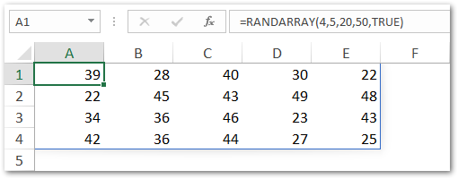
Suppose you want to return random whole numbers between 20 and 50 in a table array with 4 rows and 5 columns.
To achieve this, simply enter the following formula:
=RANDARRAY(4,5,20,50,TRUE)
As a result, excel returns whole numbers between 20 and 50 in the table having 4 rows and 5 columns. See the image below:

Note that the excel RANDARRAY function exhibits a spill behavior. The term ‘Spill’ means that when the formula has multiple outputs or results, it returns these multiple results in multiple adjacent cells (spill range).
In such a case, although the formula remains in a single cell (cell A1 above), however, the formula result spills in multiple cells or range of cells (A1:E4 above).
This new feature is only available in Office 365.

Default Values in RANDARRAY Excel Function
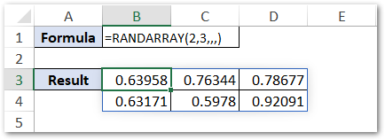
- If you do not specify the [row] and [height], the formula then returns a single random decimal value in the active cell.

- Similarly, if you keep the [min] and [max] input arguments as blank, the formula returns random decimal values between 0 and 1.

- The value of the [integer] argument is FALSE, by default. It means, if you do not specify the [integer] argument, then the formula returns random decimal values.
- Since all the input arguments of this function are optional, therefore, if you keep the function with an empty parenthesis, then formula would return a single random number between 0 and 1 in the active cell. This means it will work similarly to the RAND excel function.

It is important to note that if you specify the [min] value greater than the [max] value, then excel will return #VALUE! formula error.
Thank You 🙂
RELATED POSTS
- CHOOSE Function in Excel – Choosing Value according to Index
- SEQUENCE Function in Excel – Generate Number Series
- Excel REPT Function – Repeat Text Multiple Times in Cell
- BINOM.DIST.RANGE Function in Excel
- COLUMN Function in Excel – Get Cell Column Number
- Dynamic Array Formulas in Excel – Usage, Example, #SPILL
