In the previous blogs, we had learned how one can start automation in excel by recording a macro and then running it. We had also learned four ways to run a macro in Excel. Among these four ways, we saw how to insert a shape or a button in excel and then assign macro to it. This enabled us to instantly run our macro at a click of a mouse. Now, in continuation of our previous blogs, as we go ahead, we would unlock the technique to add the macro button on the ‘Quick Access Toolbar’ and the ‘Ribbon Tabs’.
Before starting this, let us get a brief idea about what a ‘Quick Access Toolbar’ and ‘Ribbon Tabs’ are, and what are the differences.
Quick Access Toolbar vs Ribbon in Excel
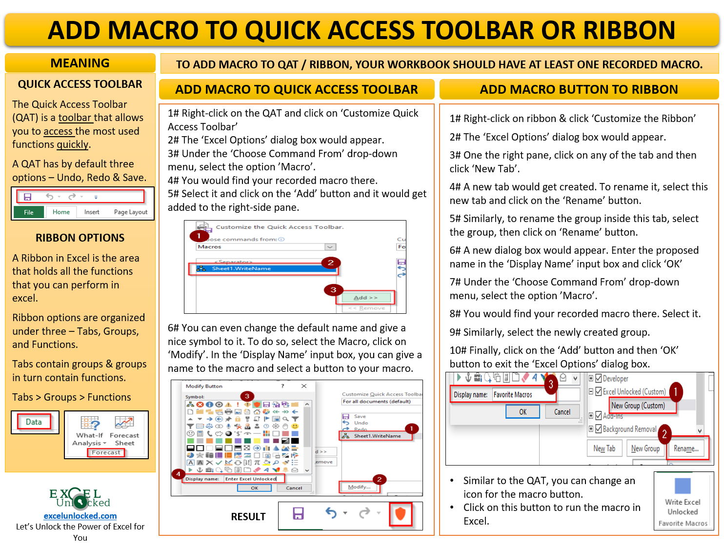
Quick Access Toolbar, as the name defines, is a toolbar in Excel which helps you to access the most used excel functions quickly. This toolbar is available on the Title Bar of the Excel workbook.
The highlighted portion in the below image is the ‘Quick Access Toolbar’.

When you install the Microsoft Excel Utility on your computer system, by default, the Quick Access Toolbar would have three buttons – Save, Undo and Redo (Refer to the image above).
Also Read: Start Automation – Record A Macro in Excel
However, you can customize the ‘Quick Access Toolbar’ according to your choice.
A Ribbon in Excel is the area that holds all the functions that you can perform in excel. The ribbon options are organized under three – Tabs, Groups, and Functions.
All the functions in excel are placed into logical groups and these groups are placed under various excel ribbon tabs.
For Example, the function ‘Text to Column’ is under the group called ‘Data Tools’. The ‘Data Tools’ group is logically placed under the tab named ‘Data’.
In the below image, you can see how the entire ribbon looks and its hierarchical structure of Tabs > Groups > Functions

Now, when you have the understanding of the Quick Access Toolbar and the Ribbon, we are good to start with learning to add the macro button to it.
Also Read: Four Ways to Run A Macro in Excel
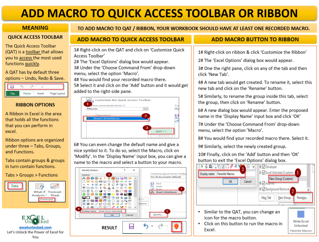
Add Macro Button to Quick Access Toolbar
Before, adding the macro button to the quick access toolbar, we need to have at least one macro inserted into our excel workbook. To insert a new quickly go through our blog on ‘Start Automation – Record A Macro in Excel’.
I have created a macro that writes the text “Excel Unlocked” in cell range A1:A5 and then changes the font formatting of the cells to Bold.
Now, when you have a macro recorded in your workbook, follow the undermentioned steps:
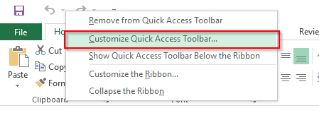
Firstly, place your mouse cursor on the quick access toolbar options, and right-click to open the list of options.
From the list that comes up, click on the ‘Customize Quick Access Toolbar’ option.
The ‘Excel Options’ dialog box would come up on your screen.
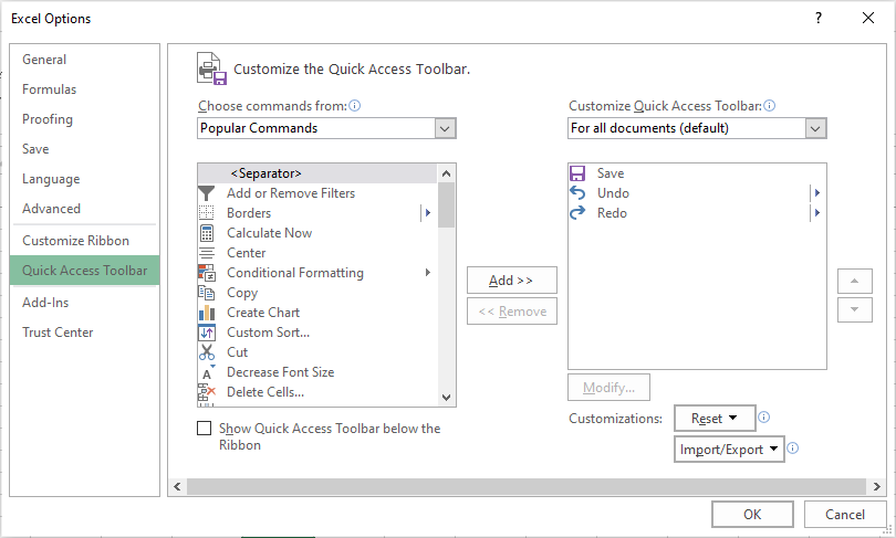
Now, click on the option ‘Macro’ from the drop-down list that appears under the section ‘Choose Command From’.
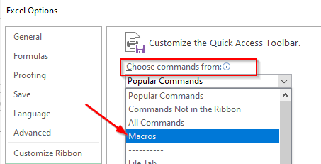
As a result, you would notice that in the box below it the recorded macro is listed (In my case it is ‘WriteName’.
If in case you have more than one macros recorded in the workbook, you would notice all of them over here.
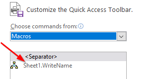
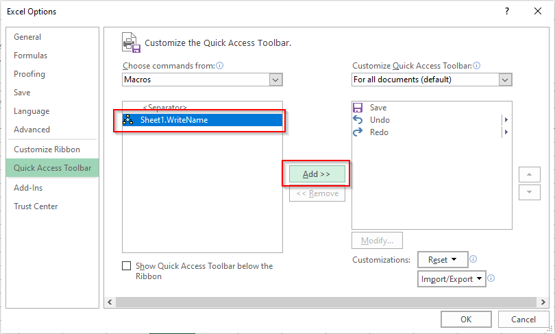
Select the macro and click on the ‘Add’ button. As a result, this would insert the macro in the right pane (below Redo function).
Now, select the macro, click on the button ‘Modify’ and choose the button of your choice.
Also, you can change the default display name, by entering some logical name to your macro button. Refer to the screenshot below:
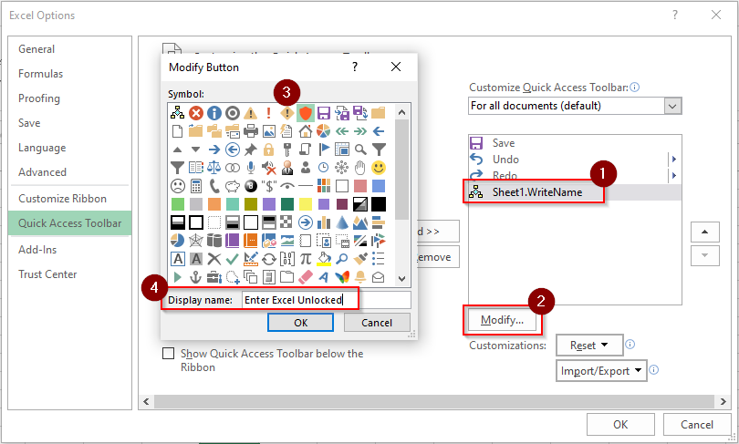
Click on OK to exit. Consequently, the excel inserts the selected macro button on quick access toolbar.

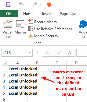
Now just click on it and you would notice that excel runs the macro.
Add Macro Button on Ribbon
You can even add the macro button on the ribbon bar in the:
- Existing Tab and New Group ; or
- New Tab
Note that you cannot add any custom option in the existing group under the existing Microsoft provided tabs.
Let us now learn this technique. In this section, we would create a new tab and add the macro button over there.
Follow the undermentioned steps:
Firstly, hover your mouse cursor on the ribbon tab and right-click to get the option.
Click on the option ‘Customize the Ribbon’.

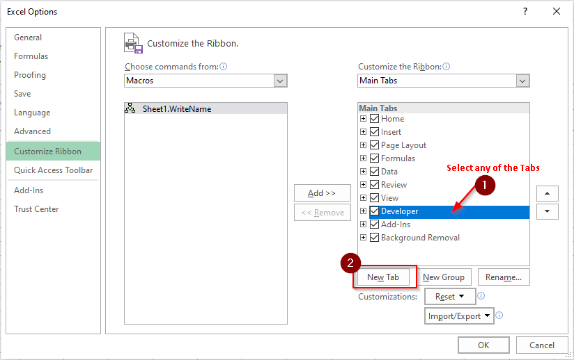
In the ‘Excel Options’ dialog box that appears, select on any of the tab names on the right pane and click on the ‘New Tab’ button.
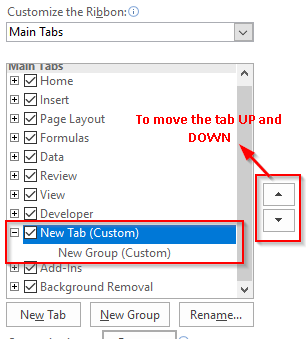
The excel inserts a new tab, having a default name as ‘New Tab (Custom)’. To change the position of this new custom tab, use the up and down buttons.
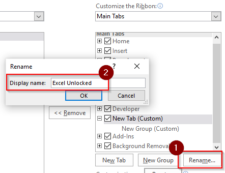
Rename this new tab using the ‘Rename’ button. Or you can right-click on the tab and click on the ‘Rename’ option. I have renamed it as ‘Excel Unlocked’.
Similarly, click on the ‘New Group (Custom)’ option under this new tab and rename it as ‘Favorite Macros’.
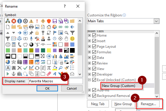
The new tab and the new group is ready now.
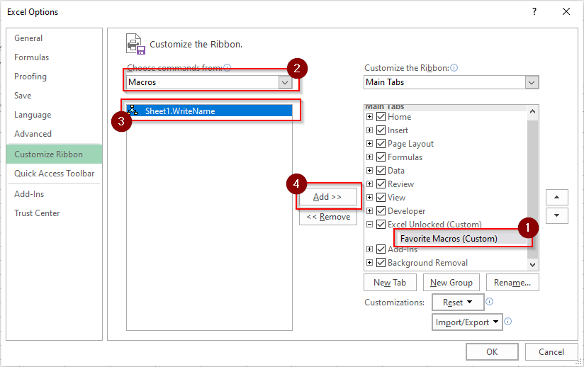
Now, firstly click on the group ‘Favorite Macros’ on the right pane. Then select the option ‘Macro’ from the drop-down list on the left pane, and select your macro.
Finally, click on the ‘Add’ button to insert the macro to this new tab under the selected group.
You can also rename and change the macro icon by selecting the macro, then clicking on the ‘Rename’ button.
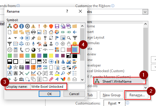
As a result, excel adds the new tab to the ribbon.

Just click on this new button and the excel would execute the assigned macro.
This brings us to the end of this blog.

