How to Unpivot Data in Excel Using Power Query

Excel Pivot Table is an amazing excel feature which is used to create different types of summary reports based on the huge table for the managerial use. However, in order to create a pivot table, you need to have the source excel table in a structured and tabular format having proper column headers. Many a time, the source table for creating pivot table is not in an appropriate tabular format. In this scenario, the unpivot table feature of the Excel power query tool would prove to be very helpful. In this blog, we would unlock the technique to unpivot excel data.

The power query feature (aka Get & Transform) is a pre-installed in Excel 2016, Excel 2019 and Office 365 excel version. However, if you are using lower excel versions, then no need to worry. There is an external power query add-in available for download from Microsoft Software Center portal. Check this tutorial.

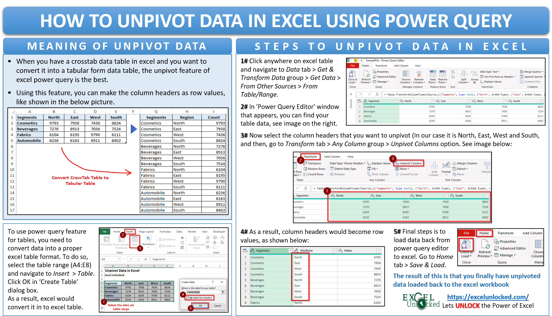
Let me first explain and make you clear about what is unpivot data and what will this feature help you to achieve at the end.

Background and Sample File – Unpivot Data in Excel

Many of the excel users have a question that how to make column headers as a row data in Excel? The answer to it is to use the unpivot data feature of Power Query.

Suppose you have a tabular data in Excel containing Segment and Region wise count of number of employees deployed in a company, as shown below:

Now, you want to convert this tabular data table into a crosstab table format as shown in the below image.

This can be easily achieved using the pivot table feature of excel. If you are enthusiastic to learn pivot table basics to advanced, you can check the Free ExcelUnlocked Pivot Table Course.

But what if you have an exactly opposite situation as that of the above. Meaning you have a crosstab table, and you want to convert it into a normal excel tabular table.

Pivot Table feature would not help in this case. Fortunately, you can use the power query feature to convert column headers as row values.

Do not confuse between the unpivot table feature of excel and the transpose feature. The Transpose feature assists you to make the table column headers as row headers and row headers as column headers. Whereas, the unpivot table feature makes column header as row values (not vice versa).

Unpivot Excel Data Using Power Query [Step by Step Guide]

Follow the undermentioned steps:

• To use the power query feature for tables, it is must to convert data into a proper excel table format. To do so, select the table range (A4:E8) and navigate to Insert > Table. Or try the Keyboard Shortcut – Ctrl + T. Click OK in the ‘Create Table’ dialog box.

• As a result, excel would convert the normal table into an excel table. Now, check below steps:

• Click anywhere on the table and navigate to the Data tab > Get & Transform Data group > Get Data > From Other Sources > From Table/Range.

• As a result, the ‘Power Query Editor’ window would pop up where you can find the table data with correctly detected column data types.

• Make sure that the excel table column headers are also promoted. If it doesn’t, then use this navigation path – Transform tab > Use First Row as Headers option.

• Now, select the column headers (keeping the Ctrl key pressed) which you want to unpivot. In our case, select column headers – North, East, West, and South.

• Then go to Transform tab > Any Column group > Unpivot Columns option. See image below:

As a result, you would notice that column headers would become row values and the number of employees data would arrange accordingly.

Let us now, change the column headers name. To change the column headers name, simply double click on the column headers. Then, write the name of your choice and then press Enter.

Final steps is to load data back from power query editor to excel. Simply go to Home tab > Save & Load.

The result of this is that you finally have unpivoted data loaded back to the excel workbook, as shown below:

What If Your Source Data Changes?

The power query feature is not just limited to performing data transformation activity. Interestingly, this feature is a dynamic feature. It is similar to the excel macro feature. Like Excel macro recorder, while you unpivot the data, the excel records and stores the steps performed by you in the form of ‘Queries and Connections’.

Suppose, in future, the original table data (crosstab table data) gets changed, or updated with some new rows of data. You can get this change/update to the unpivoted data at a single mouse click.

To understand it practically, let us take one example.

I have added four new lines of data to the crosstab table (as shown below).

This updated data does not reflect automatically in the unpivoted data. But at a click of the mouse, it is possible.

Simply, right-click on anywhere on the unpivoted table and choose the option – ‘Refresh‘. And you are done.

Consequently, power query would re-run all the steps in the backend and extract the updated data (including new rows) from the original table to the unpivoted table.

This is why power query feature became so popular. It instantly gives updated data for analysis.

With this, we have completed this tutorial on ‘How to Unpivot Data in Excel Using Power Query’. I would like hear from you in the comment box below on how did you like this blog.