The TIME Function in excel makes sure of the particular required format. Whenever we are working with time in excel, we might be willing to perform calculations on time values. Let us see how does the function work.
In this tutorial, we would learn how to use the TIME formula in excel along with some examples. This blog is an exclusive blog about the excel’s TIME function.
Here we go 😎
When To Use TIME Function of Excel
The TIME Function in Excel is useful for representing time in a format of hh:mm AM/PM. It can also convert the seconds, months into hours. The function is useful in performing arithmetic operations on time when used with other excel functions.
The TIME function belongs to date/time functions group of Excel.
Syntax and Arguments
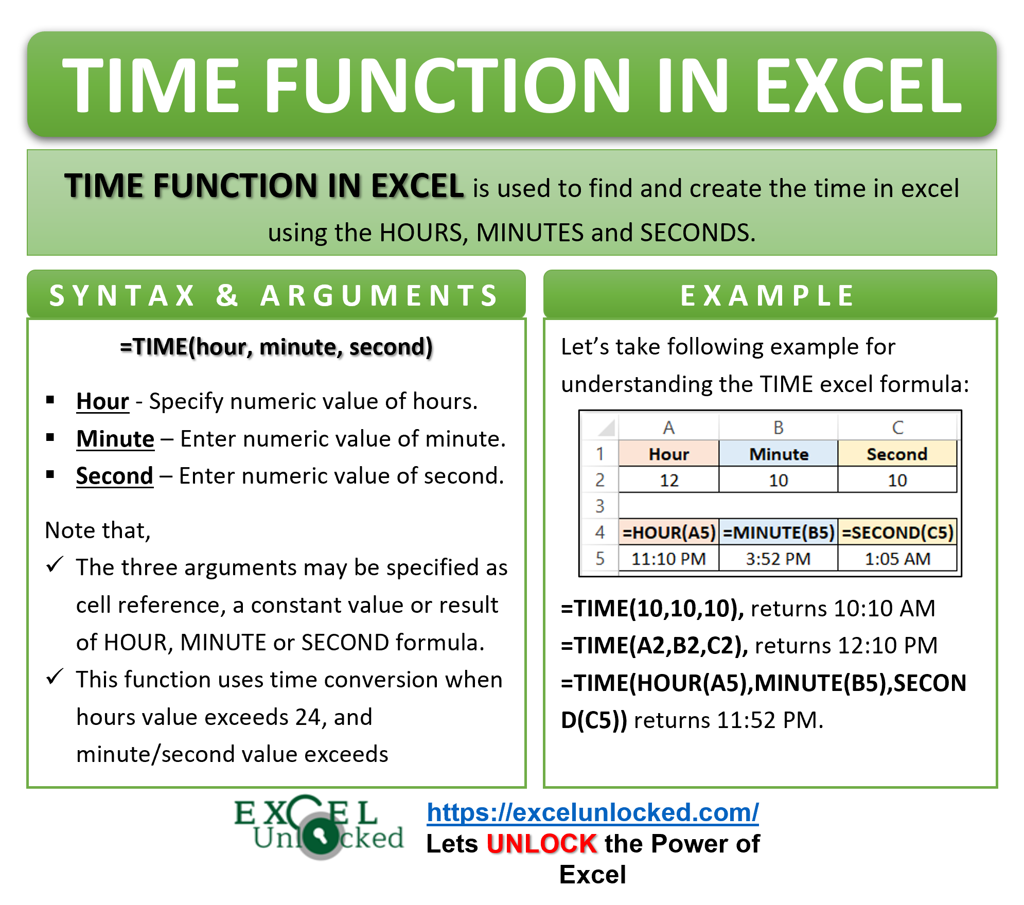
=TIME(hour,minute,second)
The following points explain the required function arguments for the TIME Function of Excel.
- hour – In this argument, specify the numeric value of the hours. It can be a cell reference, a constant value or any other function like the HOUR formula of Excel.
- minute – In this argument enter the numeric value of the minutes. This could be a cell reference, a constant numerical value or a function like the MINUTE formula of Excel.
- second – In this argument enter the numeric value of seconds. It can be a cell reference, a constant numerical value or a function like the SECOND formula of Excel.
Points To Be Noted About Excel TIME Formula
The following points are important to know before the actual usage of TIME Function in Excel.
- The TIME Function acts as a clock. Whenever the number of hours exceeds 23, the time comes back to zero. Total number of hours is divided by 24 and the remainder becomes the new value of hours.
For example, see this formula =TIME(54,00,00). Here, as the hours value is greater than 24, excel divides 54 by 24 giving the remainder as 6. Therefore, the result of the formula is 6:00 AM.
- The value of minutes and seconds argument can be greater than 60. In such scenario, the seconds are converted into minutes and give the new value of time. Similarly, the minutes are converted into hours giving us the time conversion. (see example 2 below for more detail)
For example, =TIME(01,120,00). Here, the minutes value is greater than 60. So they are converted into hours. The number of minutes 120 divides by 60 to give 2 (any remainder will be the number of minutes i.e in this case is 00). 2 adds to the hours to give 1+2=3 as the new value of hours. The result becomes 3:00 AM.
- If the value of Hours, Minutes, Seconds is greater than 32768 then the function will not give a time conversion but instead return a #NUM! error. The time conversion is only possible for values up to 32766.
- Excel performs calculations on the numerical values of time and not in the actual time format. Just like the valid dates in Excel that start from 1 Jan 1900 as 1, 2 Jan 1900 as 2. The time values start from 0 as 12:00 AM and end at 0.999988426 as 11:59 PM. Check this link for more detail about this.
Examples To Learn Usage Of Excel TIME Function
In this section of the blog, we will perform some practical examples to learn the usage of the TIME formula of Excel.
Ex. 1 – Simple Example – Using TIME Function of Excel
In this example, we will try to understand the different ways of passing the function arguments for the TIME Function. See the sample data below:

Use the following three excel formulas to use the TIME Function Excel.
=TIME(10,10,10)
=TIME(A2,B2,C2)
=TIME(HOUR(A5),MINUTE(B5),SECOND(C5))

As a result, the formula has returned 10:10 AM, 12:10 PM, 11:52 PM.
Explanation – In the first formula, we have passed 10,10,10 as the hour, minute and time respectively. So the function returns the time in format hh:mm AM/PM.
In the second formula, we have passed the cell references as the number of hours, minutes, and seconds. As a result, the function returns the time in the required format.
In the third formula, we have passed the HOUR, MINUTE, and SECOND functions of Excel as the function argument. The functions extract the value of hour from cell A5, minutes from cell B5, and second from cell C5 and return the time value as 11:52 PM.
Ex. 2 – Doing Time Conversion Using TIME Function of Excel
In this example, we will perform time conversions of seconds into minutes, minutes into hours, and hours circling back to zero after one complete day.
Below are the different values of required function arguments.

Use the following excel formula to get the results.
=TIME(A2,B2,C2)
As a result, excel returns either 12:02 AM or 00:02:00 based on the cell’s time format.

Explanation Regarding The Records
- In the first record, the number of seconds is greater than 60. Therefore, the function divides 120 by 60 and adds the resultant quotient value (i.e. 2) to the minute value, like this 0+2=2. And the remainder becomes the seconds value (i.e. 0). The result of the formula becomes 12:02 AM (hh:mm AM/PM) or 00:02:00 (hh:mm:ss)
- In the second record, the number of second is greater than 60. Therefore, the function divides 125 by 60, and adds the resultant quotient to the minute value (1+2=3). The remainder 5 becomes the value of seconds. As a result, the output is 12:03 AM or 00:03:05.
- For the third one, the number of minutes is greater than 60. Theefore, the function divides 600 by 60. The quotient (10) will be added to the number of hours (0+10) and the remainder becomes the value of number of minutes (0). As a result, the final output is 10:00 AM or 10:00:00.
- In case 4, the number of minutes is greater than 60. 650 when divided by 60, the quotient is added to the number of hours (1+10=11) and the remainder becomes the value of number of minutes (50). The result of the formula becomes 11:50 AM or 11:50:00.
- In the last record, The number of hours is greater than 24. 52 when divided by 24, the quotient will be omitted and the remainder becomes the new value of number of hours (4). The value of minutes and seconds remain unaffected. The result of the formula becomes 4:50 AM or 4:50:50.
Ex. 3 – Finding Difference in Time And Date Using The TIME Function of Excel
Surprisingly, we cannot directly use the Excel TIME function to find the time gap between starting and ending points of the time period.
In this example, we have the date and time values merged together in one cell. We need to find the time gap between the two values in days, hours, minutes, and seconds.
Below are the starting and the ending point of time in the Date Time format.

Formula used in Segments
We will start by finding the difference between two cells A2, B2. Use this formula in cell C2.
=A2-B2
We will make sure the cell format of cell C2 is “General”. We can change the cell format as explained in Example 2.
Now use the INT Formula of Excel to Extract the number of days from the result obtained in cell C2. Use this formula in cell D2.
=INT(C2)
To extract the number of hours from the difference of two date/time values, use the Excel HOUR Formula in cell E2.
=HOUR(C2)
In order to Extract the number of Minutes use this formula in cell F2.
=MINUTE(C2)
To extract the number of seconds use this formula in cell G2.
=SECOND(C2)
Combined Formula Result
Now we can simply combine the result of the four formulas using the ampersand (&). The ampersand acts as a glue, combining the result of formulas along with the text strings enclosed within the Double quotes. Use the following Formula.
=INT(C2)&" Days "&HOUR(C2)&" Hour "&MINUTE(C2)&" Minutes "&SECOND(C2)&" Seconds"

As a result, the formula has returned 233 Days 14 Hours 59 Minutes 45 Seconds.
Explanation – The difference between the two cells A2 and B2 gave the value of the gap of the time period in the number format. The number of days is represented by the part before the decimal point in C2. We have Extracted it using the INT formula of Excel ( cell D2 ).
In the same way, we have extracted the hours, minutes, and seconds from the digits after the decimal point of the numerical value in cell C2.
The result is combined with the glue called ampersand (&).
We have merged the text strings ” Days “,” Hours “,” Minutes “,” Seconds ” in between the formula results.
This brings us to the end of the function blog.
Thank you for reading 😉