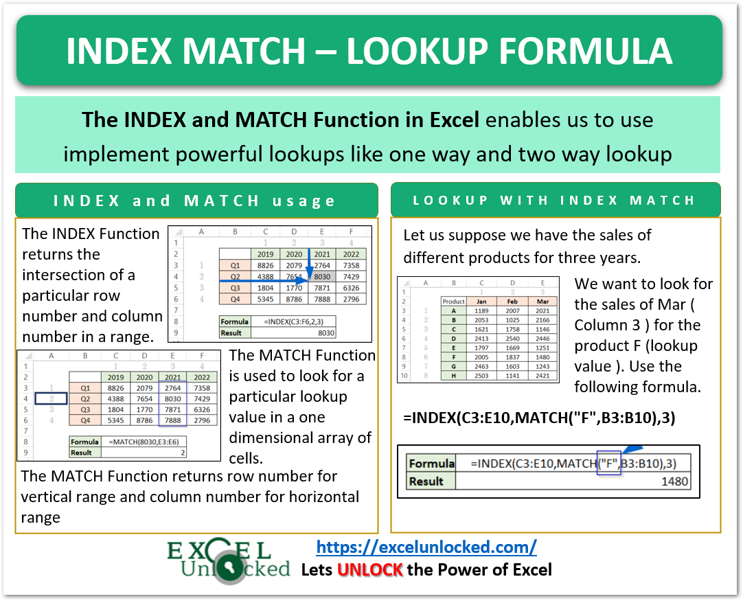
In the previous blogs, we did the usage of INDEX and MATCH Function in Excel. The combined INDEX and MATCH Function use enables us to implement powerful lookups. We can perform the one-way lookup, two-way lookup, left lookup, and more with the INDEX MATCH.
So let’s start learning.
INDEX – Get the Intersection
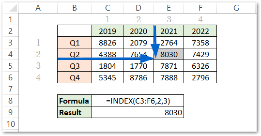
The INDEX Function gives us the intersection of a particular row and column from our range. We need to pass the following function arguments to the INDEX Function.
- array – This is the reference to the range of cells.
- row_num – This is the row number.
- [col_num] – This is an optional argument and requires the column number
=INDEX(C3:F6,2,3)
Here you can see that the intersection of the second row and the third column in the range C3:F6 gives us the sales of Quarter 2 in the year 2021 (8030).
MATCH – Finding the Cell Position
This is a lookup function. The MATCH Function gives us the position of a cell in terms of row number or column number in an array of cells. The following are the function arguments of the MATCH Function.
- Lookup_value – This is the value that we want to find in the array.
- Lookup_array – This is a one-dimensional array in which we want to search the position.
- [match_mode] – This can be 0 (exact match), 1 (less than), -1 (greater than).
=MATCH(8030,E3:E6)
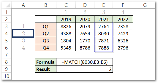
The position of 8030 in the range E3:E6 is in the second row.
We can use the MATCH Function to get the column number when we have the horizontal array of cells as follows:-
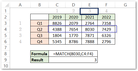
Here the lookup_array is a horizontal range of cells C4:F4 which is why the function returned column number 3 as the position of 8030 in the lookup_array.
If you need, you can see the in-depth usage of INDEX and MATCH Function in Excel
Example of One Way Lookup – INDEX and MATCH combined
Let us suppose that we have the sales of different products for three months as follows:-
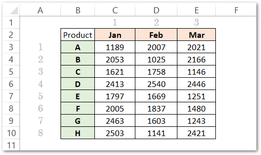
We want to get the sales of product F for March by using the following INDEX Function formula in excel.
=INDEX(C3:E10,6,3)
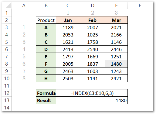
But the problem with this lookup is who wants to enter the row number and column number to just feed the INDEX Function with the location.
Why now let the MATCH function tell the INDEX Function that this is the row number of the values we are looking for?
Now replace the row argument of the INDEX Function with the MATCH Function as follows:-
=INDEX(C3:E10,MATCH("F",B3:B10),3)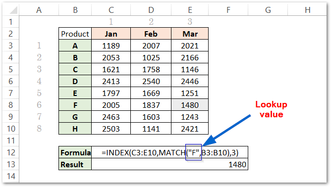
Here the MATCH Function will search for “F” ( lookup value ) in the range B3:B10 ( lookup range )and return 6 as the row number. This result of MATCH Function will further be used by the INDEX Function to return the 6th ( row number ) numbered sales value of sales in the march ( hard coded as column number 3 ) in the range C3:E10.
We can even use reference to the cell containing lookup value as:-
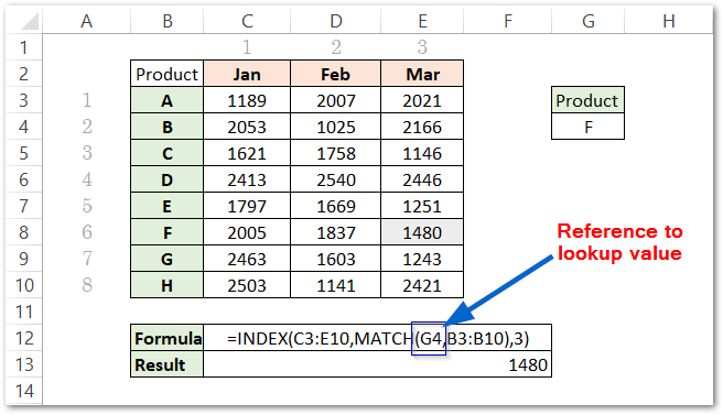
This is one way lookup as we can look for the sales of any Product ( G4 contains the Product ), but the Month is fixed as March ( column 3 hardcoded )
Two Way Lookup – INDEX and MATCH
Let us suppose that we want to find the sales of different products for any of the three months. The INDEX Function requires both the row number and column number. We are going to make the row number and column number of the INDEX function as dynamic with the use of MATCH Function.
The formula syntax for implementing a Two Way Lookup is:-
=INDEX(lookup_array,MATCH(lookup_value1,lookup_column_array),MATCH(lookup_value2,lookup_row_array )
Where the following arguments are explained as follows:-
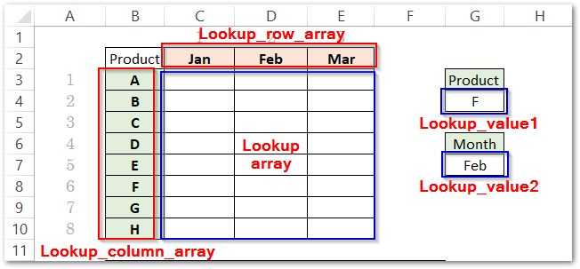
Now we can find the Sales of Product F for the month of Feb by using the following formula:-
=INDEX(C3:E10,MATCH(G4,B3:B10),MATCH(G7,C2:E2))
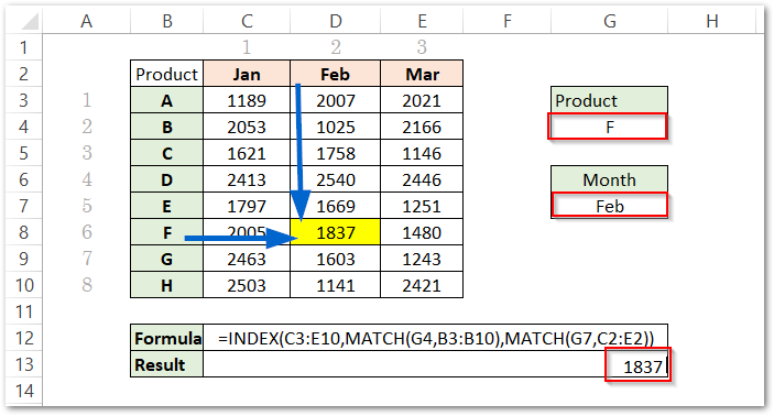
We can change the value in cells G4 (Product name ) and G7 ( Month ) to get different lookup results.
This brings us to the end of blog.
Thank you for reading.
