Many a time, it may have happened with you that you have a lot many formulas in your excel worksheet and you want to find only those cells that contain formulas. One way is to go to each and every cell one by one and then check if it contains any formula or not. But don’t you think that it is a quite time-consuming and irritating activity? Yes, it is. Indeed, there are many easy ways that you can use to find the cells containing formula at one click. In this blog, we would unlock this technique to find formula cells in Excel. There are multiple ways to achieve it.
Methods to Find Formula Cells
As mentioned in the introduction paragraph of this blog, there are mainly three ways to find all the cells that contain formula in it. Let me list those down first.
- Using the ISFORMULA function
- Using ‘Conditional Formatting’ Feature
- ‘GoTo Special’ Functionality
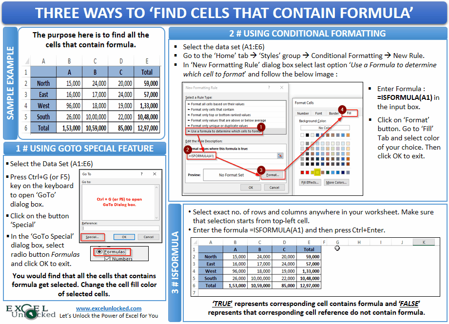
Sample Example Data
Below is the screenshot of containing sales data in a table format region wise. In this dataset, there are few cells that contain formula in it. The goal here is to find all the cell containing the formula.

Let us now start learning each of the methods one by one.
Find Formula Cells Using ISFORMULA function in Excel
In this method, we would learn how to use an excel pre-provided formula to find all the cells containing a formula in it. The formula about which I am talking about is – ‘ISFORMULA‘.
The formula nomenclature itself makes it clear that this function/formula would check if it IS a FORMULA.
Syntax and Attributes: The formula syntax goes like this: =ISFORMULA(reference); where ‘Reference’ means the reference of the cell or range.
Return Values: This formula returns ‘TRUE‘ if the reference cell contains a formula and ‘FALSE‘ in vice versa situation.
Let us now use this function in our example. Follow the below steps:
Select the exact number of cell range as that of the original data table somewhere in the worksheet. In my example, since I have the data table with 6 rows and 5 columns, therefore, I have selected exactly 6 rows and 5 columns at some other place in Excel (A5:E13). Refer to the screenshot below:

Make sure that the starting cell of the selection should be the top-left cell (in our example it is A8). As can be seen from the screenshot above, we started the selection from cell A8 and therefore, cell A8 is the active cell now.
Now, just type the formula =ISFORMULA(A1) and press Ctrl+Enter. As a result, you would notice that Excel enters the same formula in all the cells in the selected cell range.
Consequently, the formula returns TRUE and FALSE as a return value. This depicts that the reference cells corresponding to the cells with TRUE contain a formula. And the reference cells corresponding to the cells with FLASE do not contain any formula.

Using Conditional Formatting to Find Formula Cells
This method is an extension of the above method. One of the limitations of the above method is that the method does not provide the required information (that whether a cell contains a formula) in the cell itself. As you can see, the information that the cell E4 has a formula in it is provided in the cell E11 (as the return value TRUE).
To mitigate this, we can use the conditional formatting functionality along with the ISFORMULA function to find determine a formula cell (in that cell itself). Follow the procedure below:
Firstly, select the cell range (A1 to E6).
Now, navigate to the ‘Home’ tab. There you would find an option called ‘Conditional Formatting’.

Click on this feature, and select the option ‘New Rule’ from the list of a drop-down menu.

Under the ‘Select a Rule Type’ section, click on the last option ‘Use a formula to determine which cell to format’ and enter the formula =ISFORMULA(A1) in the input box available.
Next, click on the option ‘Format’ to open the ‘Format Cells’ dialog box. Under the tab named ‘Fill’, and select the cell fill color of your choice from the list of available colors (I have selected the Yellow color).

Finally, click on the ‘OK’ button to activate the format cell and then exit the ‘Conditional Formatting’ dialog box by clicking on the ‘OK’ button.
As a result, you would notice that the excel highlights all those cells that have a formula in it.
Using GoTo Special Functionality
This is yet another method to find all the cells containing the formula. This is a widely used method among all the other methods as no formula is needed to use this function. Follow the undermentioned steps-
Firstly, select the dataset table

Now press Ctrl+G key combinations on your keyboard to open the “GoTo” dialog box.
In the “GoTo” dialog box, click on the “Special” option as highlighted in the screenshot below.

The “GoTo Special” dialog box would open.

From the list of available options, click on the radio button “Formulas” and then click on the “OK” button to exit this dialog box.

As a result, you would notice that all the formula cells get selected.

Finally, just change the fill color of all those cells by choosing the color of your choice from the list of available colors. Refer to the screenshot below

You can even do any kind of formatting to these cells, like changing the font size, color, etc.
This brings us to the end of this blog. Share your views and comments in the comment section below.
RELATED POSTS
- ISNUMBER Function of Excel – Checking If Cell Contains a Number
- ISNONTEXT Function of Excel – Check Non Text Cell in Excel
- Using =IF() Function For Partial Match in Excel
- ISLOGICAL Function in Excel – Checking for Boolean TRUE/FALSE
- How to Select Cells Containing Data Validation
- SEARCH Function in Excel – Search String in Excel