AMORLINC Function of Excel – Finding the Depreciation of as Asset

Depreciation means the decreasing of the worth of an asset with time due to its wear and tear. Any valuable thing costs the original price when new, but its value decreases with time at a particular rate. In other words, we can say that the value of an asset decreases at a fixed rate annually. This is when the AMORLINC Function comes into its usage. In this tutorial, we would learn the AMORLINC function for calculating depreciation in excel.

Here we go 😎

When to Use AMORLINC Function of Excel

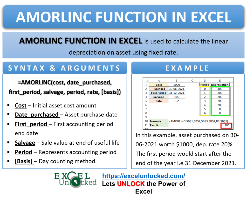
The AMORLINC function finds the depreciation of an asset for each accounting period. The function can calculate the linear depreciation at a fixed rate depending on the purchase date of the asset.

The AMORLINC function can be categorized under the Financial functions of Excel.

Syntax and Arguments

=AMORLINC(cost,date_purchased,first_period,salvage,period,rate,[basis])

The following points explain the function arguments for AMORLINC Function.

• cost – The argument refers to the value of asset at the beginning.

• date_purchased – The date on which asset was purchased.

• first_period – The date after which first period starts.

• salvage – The lowest value of asset at the end of its useful life.

• period – This refers to the accounting period.

• rate – This is the rate of depreciation.

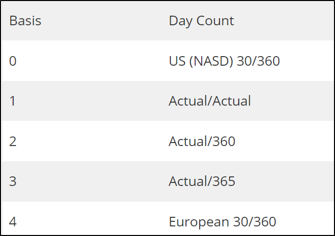
• [basis] – This is the method for day count. It is an optional argument. It can have the following values.

Points to Remember About AMORLINC Function

The following points should be kept in mind before actually using the AMORLINC function of Excel.

• The defualt value of basis is 0.

• The Accounting period starts from 0 i.e from date of purchase to the first period date.

• date_purchased and first_period must be valid excel dates. The excel dates start from 1 January 1900. All the dates before that would be invalid and return #NUM! error.

• Salvage cannot be greater than cost. In that case, AMORLINC function will return a #NUM! error.

• The depreciation is calculated without the use of depreciation coefficient.

• We can use the DATE function of Excel to get the dates in correct format for date_purchased and first_period.

Example to Learn AMORLINC Function

Let us now do some examples leading us to the practical usage of the AMORLINC Formula.

Simplest Example for AMORLINC Formula

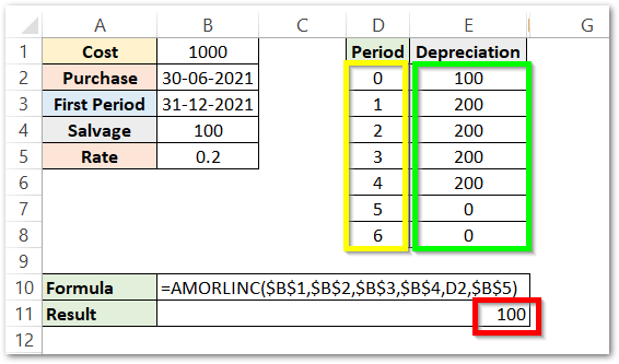
In this example, let us say an asset purchased on 30 June 2021 worth $1000 has a depreciation rate of 20%. The first period would start after the end of the year i.e 31 December 2021. The lowest value of the asset after its complete usage is $100. Below is the data:-

For easy understanding, there are two columns having names “From” and “To”. They contain the dates from where the corresponding period will start and end.

Use this formula to calculate the depreciation at the end of each of these periods.

=AMORLINC($B$1,$B$2,$B$3,$B$4,D2,$B$5)

As a result, the AMORLINC function has returned 100.

Explanation – When the value of the period is 0, it means that the first complete accounting year has not been started yet. In other words, we can say that 0 is for less than one complete year. The duration of the period ( 30 June 2021 to 31 Dec 2021) is approximately 6 months or half-year. AMORLINC function finds the 20% (0.2) amount of depreciation on the asset worth $1000.

Depreciation = cost*rate*period

= 1000*0.2*1/2

= 100

This is how the worth of assets will lower down by $100 by the end of this period.

Similarly, we can check how the depreciation is calculated for 1st accounting period.

Depreciation = cost*rate*period

= 1000*0.2*1

= 200

Therefore the worth of assets will be lower down by another $200 in the next year. In other words, we can say that the worth of assets would be $700 ( 1000-100-200 ).

Concept Behind Zero Depreciation in AMORLINC Function of Excel

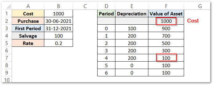
The thing to be noted here is that the depreciation amount is zero at the end of the 5th period. This is why because the salvage of assets has reached by that period. We need to calculate the value of assets at the end of each of these periods to understand the concept.

We have added a row for the cost of the asset at the beginning, Use this formula in cell F3.

=F2-E3

Now we can easily see that by the end of the 4th period, the salvage value has reached. In other words, we can say that this is the value of the asset at the end of its useful life.

If the depreciation would not be zero once the salvage is reached, then the value of the asset will become negative.

Relative and Absolute Referencing

Whenever we copy a formula, there comes a change in the cell references. The cell references move one cell down when the formula copies to the next cell. This is known as relative referencing.

We have used relative referencing for the period in the above example so that its value changes when we copy down the formula.

In absolute referencing, we lock the cell referencing so that they do not change even if we copy the formula. We have used absolute referencing for cost, date_purchased, first_period, salvage, and rate.

Thank you for reading 😉